3.5.14. SOLVE function
optional
This function is used to compute a simulation response on the model. The results obtained are stored in a solution object that can be visualized using the OUTPUT-IMAGE function.
In SesamX, a simulation is composed of multiple steps. Each step is associated with a specific physics and resolution procedure. To define a simulation scenario, you need to provide the sequence of steps that SesamX must solve. Before solving a step, SesamX initializes the step resolution using the previous step results, ensuring a perfect continuity across the steps.
This approach enables the definition of complex simulation scenarios, mixing various physics (stress, thermal, …), resolution procedures (static, transient, modal, …) and non-linearities (geometric, contact, …).
Here, we describe first the main concepts involved in a non-linear resolution procedure, and then we explain how to set up simulations using SesamX.
Non-linear resolution basics
Introduction
Before discussing non-linear analysis, let's first share some words about linear analysis. Applying the linear finite element approach to a given model leads to the following algebraic equations (written in matrix form):
$$ \lbrack K \rbrack \lbrack X \rbrack = \lbrack F \rbrack $$
Where:
- $\lbrack K \rbrack$ is the stiffness matrix (known matrix),
- $\lbrack F \rbrack$ is the force column matrix (known column matrix),
- $\lbrack X \rbrack$ is a column matrix carrying the displacements at the nodes. This column matrix is the unknown we are looking for.
Solving this kind of linear system is easy: unless the system of equations is badly conditioned (which is usually not the case for common structural application), efficient algorithms (also called linear solvers) can solve this problem with great precision. Most of all, these solvers are robust and do not ask the user to fine tune the solvers parameters to make them work correctly.
Applying a non-linear finite element approach to a given model leads to a similar system of equations, but the linearity is lost:
$$ \lbrack F_{int}(\lbrack X \rbrack) \rbrack = \lbrack F \rbrack $$
- $\lbrack F_{int}(\lbrack X \rbrack) \rbrack$ is the internal forces column matrix. It is a non-linear multi-valued function of the displacements at the nodes $\lbrack X \rbrack$,
- $\lbrack F \rbrack$ is still the force column matrix.
In the linear approach, we simply have:
$$ \lbrack F_{int}(\lbrack X \rbrack) \rbrack = \lbrack K \rbrack \lbrack X \rbrack $$
In other words, in linear analysis the internal forces is a linear function of the displacements.
Non-linear resolution procedure
However, unlike linear analysis, in non-linear analysis we cannot obtain a closed-form solution of the problem. We must employ an iterative resolution procedure to converge to the problem solution. Multiple iterative resolution procedures exist for solving non-linear problems. The procedure mostly used for solving structural problems is the Newton-Raphson method.
The basic idea behind this procedure is to linearize the problem around the current displacement, solve this linearized problem, check if the convergence is reached, if not, repeat the procedure until the convergence is reached.
The Newton-Raphson method is quite efficient for solving structural non-linear problems because:
- Even though we do not know the solution in closed form, we know exactly the internal forces function and its first derivative (also called the tangent stiffness, as explained below).
- By splitting the non-linear problem resolution in a sequence of multiple linear problems, we can benefit from the efficient and robust linear solvers already available.
This Newton-Raphson procedure is illustrated with the following figures in the 1-dimensional case.
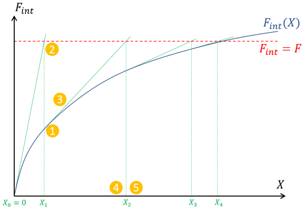
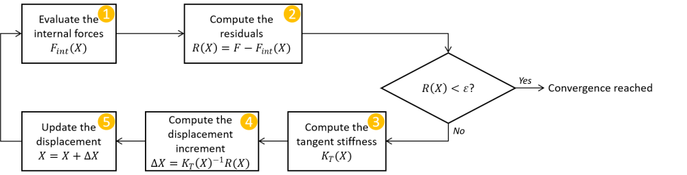
To stop the procedure, it is important to define a convergence criteria. In the example above, it is denoted as $\varepsilon$: once the residuals are small enough, the displacement is considered as converged and becomes the solution of the problem. The user must provide the convergence criteria.
Once the problem is linearized at the current displacement, it is quite similar to a linear problem. For this reason, we use the term tangent stiffness to denote the linear operator of the system. The linearization procedure is called the factorization of the problem. The factorization is often computationally expensive to perform. Hence, the tangent stiffness' inverse is not always computed from scratch at each iteration, but updated intelligently based on the previous residuals and displacement increments (using the BFGS procedure for instance). Of course this update procedure is not exact but more efficient than a full factorization. SesamX automatically analyzes the resolution progress to decide when to perform a full factorization of the problem and when to perform a simple update.
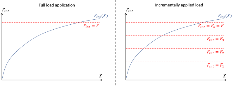
As illustrated in the previous figures, the non-linear resolution procedure is path-dependent. Indeed it follows the internal forces path to the externally applied load level. If this path is chaotic, the convergence may be difficult to reach. Most of the time, convergence issues can be avoided if the externally applied load is indeed applied incrementally. Instead of solving the system response once for the full load, the system is solved multiple times for a new load increment. Therefore, the resolution is split into multiple sub-resolutions (also called levels).
Function description
The SOLVE function allows to define a simulation scenario. You can include geometric non-linearity in your simulation with the GEOM-NL keyword.
Keywords
| Name | Data Type | Data number | Optional | Default value | Physical quantity |
|---|---|---|---|---|---|
| MODEL | STRING | 1 | NO | ||
| Name of the model on which to compute the non-linear resolution. | |||||
| NAME | STRING | 1 | NO | ||
| Name of the resulting solution object. | |||||
| GEOM-NL | BOOLEAN | 1 | YES | YES | |
| Boolean to activate the geometric non-linearity. | |||||
STEPS branch
mandatory unique
The STEPS branch is used to specify the sequence of steps that SesamX must compute. The following links guide you to the documentation related to each type of step supported by SesamX:
- STATIC-STRESS: static-stress resolution step.
Examples
Multi steps simulation
The following example showcases how to set up a simulation composed of multiple steps (here 2 static-stress steps).
SOLVE
  NAME: NL_ANALYSIS
  MODEL: PIPE_CRUSHING
  GEOM-NL: YES

  STEPS
    STATIC-STRESS
      NAME: LOADING
      NB-LEVELS: 10
      CONSTRAINTS
        - NAME: BOUND_CASE  AMPLITUDE-FUNCTION: "1"
      LOADS
        - NAME: LOAD_CASE  AMPLITUDE-FUNCTION: "t."
      CONTACT: CONTACT_CASE

    STATIC-STRESS
      NAME: UNLOADING
      NB-LEVELS: 10
      CONSTRAINTS
        - NAME: BOUND_CASE  AMPLITUDE-FUNCTION: "1"
      LOADS
        - NAME: LOAD_CASE  AMPLITUDE-FUNCTION: "1-t."
      CONTACT: CONTACT_CASE
See also
References
-