The beam finite element is one the main elements proposed by structural finite element analysis software. This element deserves a full article to explain what it is about. I will focus on the Timoshenko beam element because it is the most common beam element implemented in FEA software. First, I will expose the assumptions underlying this element, as well as how to derive the beam element stiffness matrix. Finally, I will conclude this article with an example of a cantilever beam model simulated using the SesamX finite element analysis software.
Quick remark on notations
Before starting, let’s define some notations that are used through this article:
vectors are denoted with an underline $ \underline{u} $ ,
matrices are represented with brackets $ \lbrack \ \rbrack $ ,
Einstein summation convention is used on repeated indices,
partial derivatives are denoted with the comma notation $ u_{,x} $ ,
infinitesimal strain and stress tensors are represented in column matrix notation $ \lbrack \varepsilon \rbrack = \begin{bmatrix} \varepsilon_{11} \\ \varepsilon_{22} \\ \varepsilon_{33} \\ \varepsilon_{12} \\ \varepsilon_{23} \\ \varepsilon_{13} \end{bmatrix} $ and $ \lbrack \sigma \rbrack = \begin{bmatrix} \sigma_{11} \\ \sigma_{22} \\ \sigma_{33} \\ \sigma_{12} \\ \sigma_{23} \\ \sigma_{13} \end{bmatrix} $ , where $ \lbrack \varepsilon \rbrack $ represents the engineering strains.
Introducing the beam element
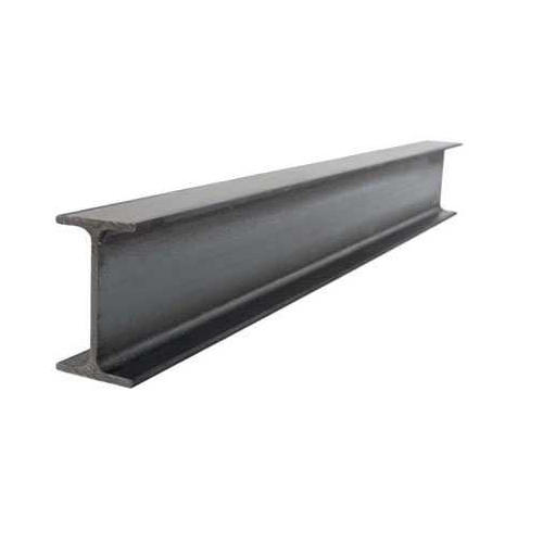
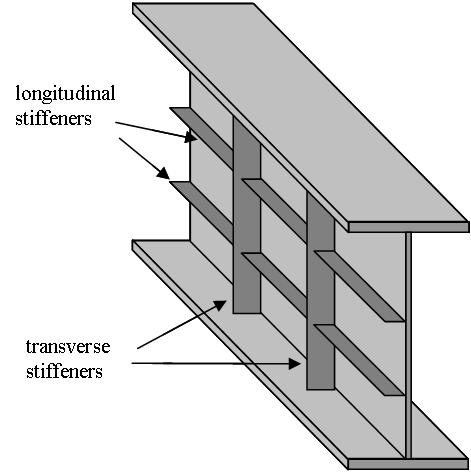
The beam element is relevant to use when we aim at analyzing a slender structure undergoing forces and moments in any direction. For instance, it makes it the perfect element to analyze the support of a slab or a plate stiffener.
 |
 |
|---|---|
A beam can be more simplistically represented as follows.
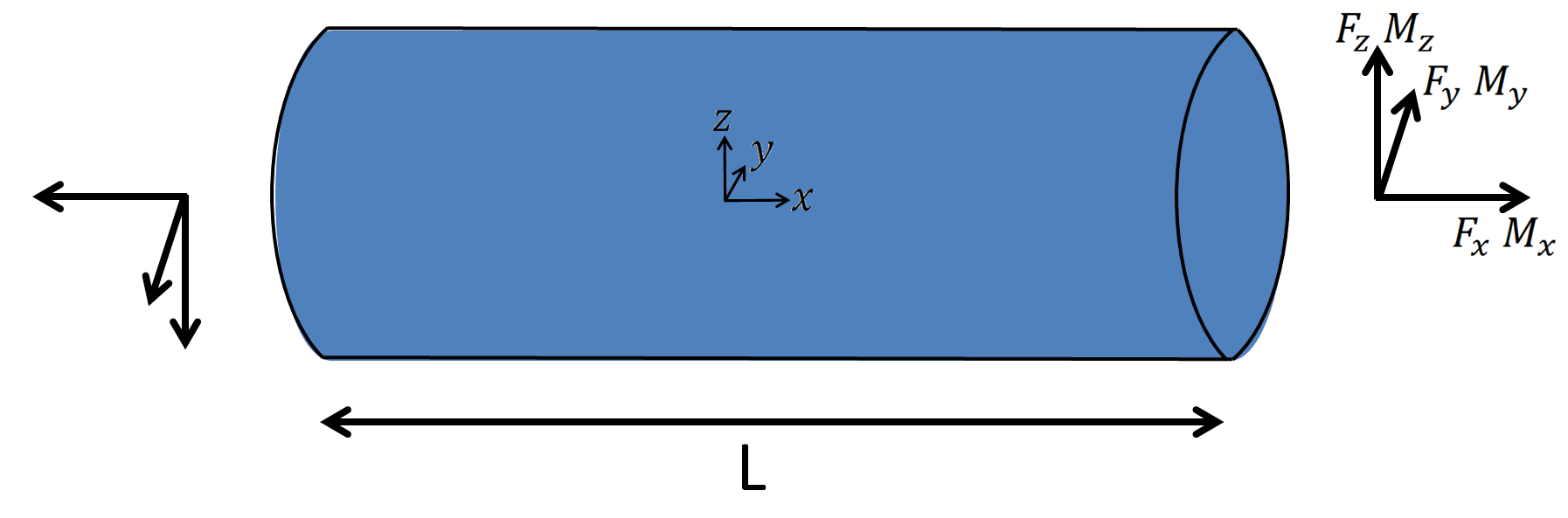
We are interested here in a beam whose neutral axis is the same as the shear axis. In other words, bending is supposed uncoupled from shearing. From beam theory (or as it will appear during the following derivation), the relevant geometric parameters of the beam are:
The length of the beam: $ L $
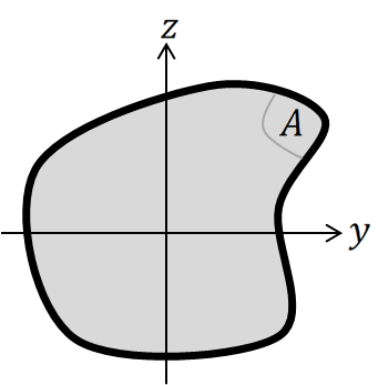
The area of the beam cross-section: $ A $
The area moments of inertia of the beam cross-section:
$$ I_y = \iint_A z^2 dydz $$
$$ I_z = \iint_A y^2 dydz $$
The product moment of inertia of the beam cross-section:
$$ I_{yz} = \iint_A yz dydz $$
The polar moment of inertia:
$$ I_{x} = \iint_A (y^2 + z^2) dydz $$
Timoshenko beam element assumptions
We can view a beam element as a simplification of a more complex 3D structure. When designing such an element, the aim is to decrease the computational cost, while making relevant assumptions on how the element behaves. The main assumptions behind the Timoshenko beam element are given here with some explanations.
1. Stress assumption
As the beam must be able to sustain transverse loading, the stress state must allow for shear stress, as well as axial stress in order to sustain bending and axial loading. It is then sufficient to enforce:
$$ \sigma_{22} = \sigma_{33} = \sigma_{23} = 0 \tag{1} $$
Remark that unlike the truss element, the beam element makes no assumption about the shear stresses $ \sigma_{12} $ and $ \sigma_{13} $ .
2. Kinematic assumption
The main assumption associated to the beam element, is that beam cross section remains straight during deformation. However, the Timoshenko beam theory does not enforce that a surface normal to the beam neutral axis remains normal during the deformation (as in classical Bernoulli beam theory).
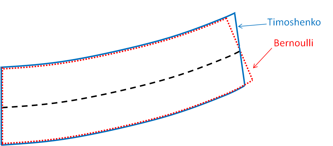
Timoshenko beam is preferred because it makes looser assumptions on the beam kinematics. In fact, Bernoulli beam is considered accurate for cross-section typical dimension less than 1⁄15 of the beam length. Whereas Timoshenko beam is considered accurate for cross-section typical dimension less than 1⁄8 of the beam length.
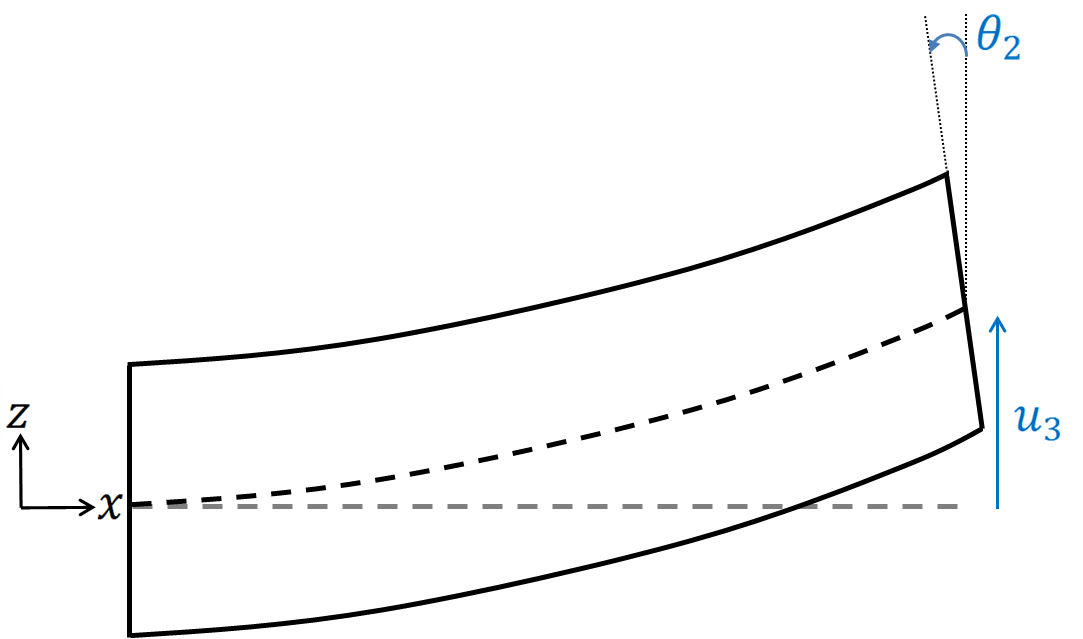
The displacement inside the beam is defined from the displacements on the neutral axis $ u_1^0(x), u_2^0(x), u_3^0(x) $ , as well as the cross-section rotations $ \theta_1(x), \theta_2(x), \theta_3(x) $ :
$$ \underline{u} = \begin{cases} u_1(x, y, z) = u_1^0(x) + z\theta_2(x) - y\theta_3(x) \\ u_2(x, y, z) = u_2^0(x) - z\theta_1(x) \\ u_3(x, y, z) = u_3^0(x) + y\theta_1(x) \tag{2} \end{cases} $$
Once we know the displacements and rotations on the beam axis, we can compute the displacement over the whole beam. Therefore, the beam element is a 1-dimensional element. The element presented here is the linear beam element. Hence, this element consist of 2 nodes connected together through a segment.
We can see from the assumed displacement given in (2), that it does not take into account the warping effect of beams with non circular cross-section. To approximately account for this effect, we can simply replace the beam polar inertia with the beam torsion constant in our equations, leaving our assumptions unchanged. The link provided previously explains how to compute the torsion constant, given the cross-section dimensions.
3. Inertia assumption
We make the assumption that the beam cross-section principal axes are along the $ y $ and $ z $ axis. Which translate, to
$$ I_{yz} = 0 \tag{3} $$
Beam element derivation
As mentioned previously, we can represent the beam element as shown in the following figure, with its local axis system.
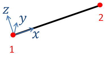
The element local axis system is defined by the axis $ (x, y, z) $ whose basis vectors are respectively denoted as $ \underline{e_{1}^{elem}}, \underline{e_{2}^{elem}}, \underline{e_{3}^{elem}} $ . (Here $ x $ is directed from node 1 to node 2 however in SesamX the user is free to chose this orientation).
The translational and rotational degrees of freedom are required on each node of the element. Hence, the displacement vector on node $ I $ will be denoted $ \underline{u^I} = {u_j}^I \underline{e_{j}^{elem}} $ , and the rotation vector will be denoted $ \underline{\theta^I} = {\theta_j}^I \underline{e_{j}^{elem}}$ where $ I $ takes the values 1 or 2.
Applying the classical finite element method we can derive the beam element stiffness matrix.
Strain tensor
The displacements and rotations are known at the nodes. To get the displacements and rotation inside the element (but still on the neutral axis) we interpolate linearly the quantities at the nodes:
$$ \begin{cases} \begin{aligned} {u^0_j}(x) &= N^I(x) {u_j}^I \\ {\theta_j}(x_1) &= N^I(x) {\theta_j}^I \end{aligned} \end{cases} $$
Where the $ N^I $ represent the shape functions of the element:
$$ \begin{cases} N^1(x) = 1 - \cfrac{x}{L} \\ N^2(x) = \cfrac{x}{L} \end{cases} $$
Using assumption (2) we can then compute the strains:
$$ \lbrack \varepsilon \rbrack = \begin{bmatrix} \varepsilon_{11} \\ \varepsilon_{22} \\ \varepsilon_{33} \\ \varepsilon_{12} \\ \varepsilon_{23} \\ \varepsilon_{13} \end{bmatrix} = \begin{bmatrix} u^0_{1,x} + z\theta_{2,x} - y\theta_{3,x} \\ 0 \\ 0 \\ u^0_{2,x} - z\theta_{1,x} - \theta_{3} \\ 0 \\ u^0_{3,x} + y\theta_{1,x} + \theta_{2} \end{bmatrix} $$
Since the actual shear strain in the beam is not constant over the cross-section, Timoshenko beam theory usually introduces shear correction factors (depending on the cross-section shape) $ k_2 $ and $ k_3 $ on $ \varepsilon_{12} $ and $ \varepsilon_{13} $ .
To make things easier, we define the following quantities:
the curvatures $ \kappa_1 = \theta_{2,x} $ and $ \kappa_2 = \theta_{3,x} $
the shear strains $ \gamma_1 = u_{2,x} - \theta_3 $ and $ \gamma_2 = u_{3,x} + \theta_2 $
the axial strain $ \varepsilon_{ax} = u_{1,x} $
the twist $ \psi = \theta_{1,x} $
And rewrite the strains as:
$$ \lbrack \varepsilon \rbrack = \begin{bmatrix} \varepsilon_{11} \\ \varepsilon_{22} \\ \varepsilon_{33} \\ \varepsilon_{12} \\ \varepsilon_{23} \\ \varepsilon_{13} \end{bmatrix} = \begin{bmatrix} \varepsilon_{ax} + z\kappa_1 - y\kappa_2 \\ 0 \\ 0 \\ k_2\gamma_1 - z\psi \\ 0 \\ k_3\gamma_2 + y\psi \end{bmatrix} \tag{4} $$
Where the curvatures, shear strains, axial strain and twist are provided with the help of the shape functions:
$$ \begin{aligned} \kappa_1 &= N^I_{,x} {\theta_2}^I \\[5pt] \kappa_2 &= N^I_{,x} {\theta_3}^I \\[5pt] \gamma_1 &= N^I_{,x} {u_2}^I - N^I {\theta_3}^I \\[5pt] \gamma_2 &= N^I_{,x} {u_3}^I + N^I {\theta_2}^I \\[5pt] \varepsilon_{ax} &= N^I_{,x} {u_1}^I \\[5pt] \psi &= N^I_{,x} {\theta_1}^I \end {aligned} \tag{5} $$
Stress tensor
To relate the stresses to the strains we need to apply Hooke’s law for linear elastic material.
$$ \begin{bmatrix} \varepsilon_{11} \\ \varepsilon_{22} \\ \varepsilon_{33} \\ \varepsilon_{12} \\ \varepsilon_{23} \\ \varepsilon_{13} \end{bmatrix} = \frac{1}{E} \begin{bmatrix} 1 && -\nu && -\nu && 0 && 0 && 0 \\ -\nu && 1 && -\nu && 0 && 0 && 0 \\ -\nu && -\nu && 1 && 0 && 0 && 0 \\ 0 && 0 && 0 && 2+2\nu && 0 && 0 \\ 0 && 0 && 0 && 0 && 2+2\nu && 0 \\ 0 && 0 && 0 && 0 && 0 && 2+2\nu \end{bmatrix} \begin{bmatrix} \sigma_{11} \\ \sigma_{22} \\ \sigma_{33} \\ \sigma_{12} \\ \sigma_{23} \\ \sigma_{13} \end{bmatrix} \\ $$
Using assumption (1) on the right hand side, as well as the result we got in (4) on the left hand side, leads to a peculiar relation:
$$ \underbrace{ \begin{bmatrix} \varepsilon_{ax} + z\kappa_1 - y\kappa_2 \\ 0 \\ 0 \\ k_2\gamma_1 - z\psi \\ 0 \\ k_3\gamma_2 + y\psi \end{bmatrix} }_{\text{kinematic assumption}} = \underbrace{ \frac{1}{E} \begin{bmatrix} \sigma_{11} \\ -\nu\sigma_{11} \\ -\nu\sigma_{11} \\ (2+2\nu)\sigma_{12} \\ 0 \\ (2+2\nu)\sigma_{13} \end{bmatrix} }_{\text{stress assumption}} $$
As for the the truss element, this relation cannot hold. However using a similar explanation, we can find a way out. When making the kinematic assumption we were interested in the macroscopic behavior of the beam. Whereas the stress assumption relates more to a microscopic behavior. It turns out that even if $ \varepsilon_{22} $ and $ \varepsilon_{33} $ are not 0 (microscopic scale) their effect on the displacement (macroscopic scale) is negligible compare to what comes from the $ \varepsilon_{11}, \varepsilon_{12}, \varepsilon_{13} $ terms. Of course, this explanation becomes questionable as the slenderness of the beam degrades.
We can then simplify this relation and write:
$$ \begin{bmatrix} \varepsilon_{ax} + z\kappa_1 - y\kappa_2 \\ 0 \\ 0 \\ k_2\gamma_1 - z\psi \\ 0 \\ k_3\gamma_2 + y\psi \end{bmatrix} = \frac{1}{E} \begin{bmatrix} \sigma_{11} \\ 0 \\ 0 \\ (2+2\nu)\sigma_{12} \\ 0 \\ (2+2\nu)\sigma_{13} \end{bmatrix} $$
And we can invert it to get the stresses from the strains:
$$ \begin{bmatrix} \sigma_{11} \\ \sigma_{12} \\ \sigma_{13} \end{bmatrix} = \begin{bmatrix} E && 0 && 0 \\ 0 && \cfrac{E}{2(1+\nu)} && 0 \\ 0 && 0 && \cfrac{E}{2(1+\nu)} \end{bmatrix} \begin{bmatrix} \varepsilon_{ax} + z\kappa_1 - y\kappa_2 \\ k_2\gamma_1 - z\psi \\ k_3\gamma_2 + y\psi \end{bmatrix} $$
Beam element stiffness matrix
The element stiffness matrix is obtained through the expression of the virtual work. Denoting the virtual strains as $ \lbrack \overline{\varepsilon} \rbrack $ we have for the virtual work over the element volume:
$$ \overline{W} = \iiint_V \lbrack \overline{\varepsilon} \rbrack^T \lbrack \sigma \rbrack dV $$
After expanding we get:
$$ \begin{alignedat}{3} \overline{W} &= &E\iiint_V &\lbrack \overline{\varepsilon_{ax}}\varepsilon_{ax} + z^2 \overline{\kappa_1}\kappa_1 + y^2 \overline{\kappa_2}\kappa_2 + \overline{\varepsilon_{ax}}(z\kappa_1 - y\kappa_2) + \\ &&& (z\overline{\kappa_1} - y\overline{\kappa_2})\varepsilon_{ax} - zy \overline{\kappa_1} \kappa_2 - yz \overline{\kappa_2} \kappa_1 \rbrack dV \\ &+&\cfrac{E}{2(1+\nu)} \iiint_V &\lbrack k_2\overline{\gamma_1}\gamma_1 + z^2 \overline{\psi}\psi - z \overline{\gamma_1}\psi - k_2z \overline{\psi}\gamma_1 \rbrack dV \\ &+&\cfrac{E}{2(1+\nu)} \iiint_V &\lbrack k_3\overline{\gamma_2}\gamma_2 + y^2 \overline{\psi}\psi + y \overline{\gamma_2}\psi + k_3y \overline{\psi}\gamma_2 \rbrack dV \end{alignedat} $$
Using the fact that the beam is meshed on its neutral axis ($ \iiint_V zdV = \iiint_V ydV =0 $ ) and the inertia assumption (3), we can simplify this expression:
$$ \begin{alignedat}{4} \overline{W} &=& EA\int_L &\overline{\varepsilon_{ax}}\varepsilon_{ax} dx &\to \textbf{axial contribution} \\ &+& \cfrac{EI_x}{2(1+\nu)} \int_L &\overline{\psi}\psi dx &\to \textbf{twist contribution} \\ &+& E\int_L & \lbrack I_y \overline{\kappa_1}\kappa_1 dx + I_z \overline{\kappa_2}\kappa_2 \rbrack dx &\to \textbf{bending contribution} \\ &+& \cfrac{EA}{2(1+\nu)} \int_L & \lbrack k_2 \overline{\gamma_1}\gamma_1 + k_3 \overline{\gamma_2}\gamma_2 \rbrack dx &\to \textbf{shear contribution} \end{alignedat} $$
Before we compute the integral, it is interesting to analyse the polynomial order of each integrand:
the axial, twist and bending integrands are of order 0, because they introduce only the $ N^I_{,x} N^J_{,x} $ products,
the shear integrand is of order 2, because it introduces the $ N^I N^J $ products (as well as the $ N^I_{,x} N^J_{,x} $ products).
For reasons not explained here, we can show that if the shear terms are integrated exactly, it will lead to element shear locking: the element will display a very stiff behavior as the length decreases. To avoid this phenomenon we degrade the shear terms integration (called reduced integration). The 1 point Gaussian integration rule integrates exactly polynomials up to the order 1. Thus using this rule, we will integrate exactly the axial, twist and bending integrands and we will reduce the integration on the shear terms.
Eventually, using (5), we can relate each of the terms obtained to the nodes displacements and rotations.
Example of a simple structure using beam elements
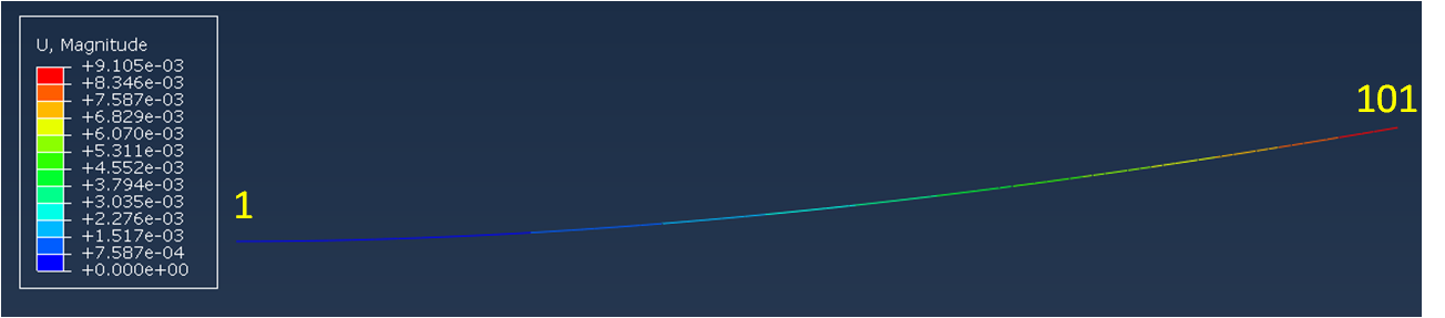
As an example, the following cantilever beam model is set up and simulated with the SesamX finite element software.
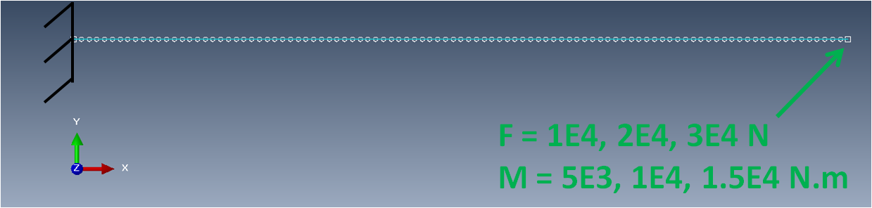
The beam is $ 1 m $ long. It is made of 101 nodes and 100 elements. The beam orientation is such that it is exactly aligned with the global coordinate system. The beam properties come from a square section of $ 10 cm $ side:
- area of $ 10000 mm^2 $
- $ J = 1.406e7 mm^4 $
- $ I22 = I33 = 8.33e6 mm^4 $
- $ K2 = K3 = 0.44 $
A linear elastic material is applied with $ E = 200 GPa $ and $ \nu = 0.33 $ . The far left node is clamped while, arbitrary force and moment vectors are applied at the other end.
This case is then solved with a linear static resolution.
And the following figure gives an overview of the displacement of the model, as well as the node numbers.
To reproduce this simulation on your own, you need:
- at least the free version of the SesamX software installed,
- the beam model mesh (in Abaqus format),
- and the SesamX input cards (defining the element properties, the loading and so on).
If you are looking to extend this example, you can get help from the SesamX documentation.
Conclusion
I hope this article has provided you a better understanding of the beam finite element. If you are looking for more information, do not hesitate to send me and email.
Did you like this content?
Register to our newsletter and get notified of new articles