When talking about structural finite elements, the truss element is one of the first elements discussed. As long as the assumptions underlying its usage are met, it is an efficient element allowing convenient interpretation of results. I will discuss here theses assumptions as well as the truss element use cases. Then I will showcase the element formulation, leading to the expression of the truss stiffness matrix, as it is commonly implemented in finite element analysis software. Finally, I will conclude this article with an example of a truss assembly simulated using the SesamX finite element analysis software.
Quick remark on notations
Before starting, let’s define some notations that are used through this article:
vectors are denoted with an underline $ \underline{u} $ ,
matrices are represented with brackets $ \lbrack \ \rbrack $ ,
Einstein summation convention is used on repeated indices,
partial derivatives are denoted with the comma notation $ u_{,x} $ ,
infinitesimal strain and stress tensors are represented in column matrix notation $ \lbrack \varepsilon \rbrack = \begin{bmatrix} \varepsilon_{11} \\ \varepsilon_{22} \\ \varepsilon_{33} \\ \varepsilon_{12} \\ \varepsilon_{23} \\ \varepsilon_{13} \end{bmatrix} $ and $ \lbrack \sigma \rbrack = \begin{bmatrix} \sigma_{11} \\ \sigma_{22} \\ \sigma_{33} \\ \sigma_{12} \\ \sigma_{23} \\ \sigma_{13} \end{bmatrix} $ , where $ \lbrack \varepsilon \rbrack $ represents the engineering strains.
Introducing the truss element assumptions
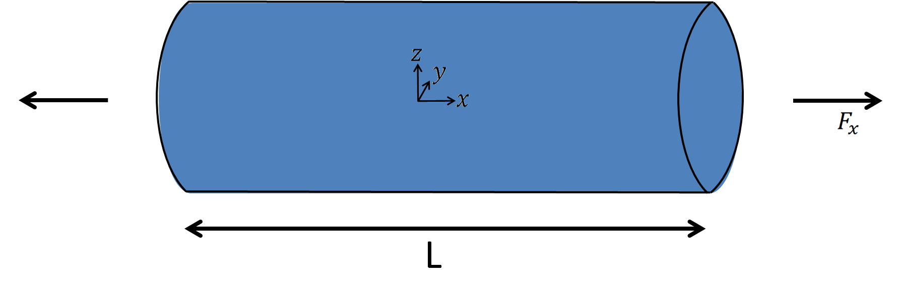
The truss element is relevant to use when we aim at analyzing a slender structure which only undergoes axial loading.
For such a structure, the axial stress assumption is commonly used:
$$ \sigma_{22} = \sigma_{33} = \sigma_{12} = \sigma_{23} = \sigma_{13} = 0 \tag{1} $$
$$ u_{i,y} = u_{i,z} = 0 \tag{2} $$
(1) is also called the stress assumption and (2) the kinematic assumption. These assumptions are considered valid for cross-section typical dimension less than 1⁄10 of the truss length.
Stresses that are orthogonal to the truss axis are considered null as well as the dependence of the displacement on $ y $ and $ z $ . Thus, knowing the displacement on the truss axis is enough to describe the displacement over the whole structure: the truss element is a 1-dimensional element.
As it will appear during the stiffness matrix derivation, the relevant geometric parameters of the truss are:
the length of the truss $ L $ ,
and the area of the truss section $ A $ .
In its more simple formulation (presented here), it consists of 2 nodes connected together through a segment, yielding a linear displacement interpolation inside the element.
Assembling trusses is useful to modelize bars connected to each other by mean of pin joints, like in a crane or a bridge.

Truss element derivation
As mentioned previously, we can represent the truss element as shown in the following figure, along with its local basis vectors.
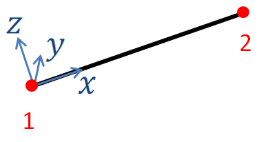
The element local axis system is defined by the axis $ x, y, z $ whose basis vectors are respectively denoted as $ \underline{e_{1}}, \underline{e_{2}}, \underline{e_{3}} $ .
Only the translational degrees of freedom are required on each node of the element. Hence, the displacement on node $ I $ will be denoted $ \underline{u^I} = {u_j}^I \underline{e_{j}} $ , where $ I $ takes the values 1 or 2.
Applying the classical finite element method we can derive the truss element stiffness matrix.
Strain tensor
Using assumption (2) the displacement inside the element can be written:
$$ \underline{u} = \begin{cases} u_1(x) \\ u_2(x) \\ u_3(x) \end{cases} $$
However, the only known information is at the node. To get the displacement inside the element we interpolate linearly the nodes displacements as follows:
$$ {u_j}(x_1) = N^I(x) {u_j}^I \tag{3} $$
Where the $ N^I $ represent the shape functions of the element:
$$ \begin{cases} N^1(x) = 1 - \cfrac{x}{L} \\ N^2(x) = \cfrac{x}{L} \end{cases} $$
Next, we simply compute the strains by differentiation:
$$ \lbrack \varepsilon \rbrack = \begin{bmatrix} \varepsilon_{11} \\ \varepsilon_{22} \\ \varepsilon_{33} \\ \varepsilon_{12} \\ \varepsilon_{23} \\ \varepsilon_{13} \end{bmatrix} = \begin{bmatrix} u_{1,x} \\ 0 \\ 0 \\ u_{2,x} \\ 0 \\ u_{3,x} \end{bmatrix} $$
However, we want the truss element to be sensitive only to axial strain. We can simply enforce other strains to be 0. Physically this means that even if there are some $ u_2 $ and $ u_3 $ displacements in the element, they do not contribute to the strain state of the element. Hence, we have:
$$ \lbrack \varepsilon \rbrack = \begin{bmatrix} \varepsilon_{11} \\ \varepsilon_{22} \\ \varepsilon_{33} \\ \varepsilon_{12} \\ \varepsilon_{23} \\ \varepsilon_{13} \end{bmatrix} = \begin{bmatrix} u_{1,x} \\ 0 \\ 0 \\ 0 \\ 0 \\ 0 \end{bmatrix} $$
Finally, using (3) we get the strains in the element from the displacements at
the nodes:
$$ \lbrack \varepsilon \rbrack = \begin{bmatrix} N^I_{,x} {u_1}^I \\ 0 \\ 0 \\ 0 \\ 0 \\ 0 \end{bmatrix} \tag{4} $$
Stress tensor
To relate the stresses to the strains we need to apply Hooke’s law for linear elastic material.
$$ \begin{bmatrix} \varepsilon_{11} \\ \varepsilon_{22} \\ \varepsilon_{33} \\ \varepsilon_{12} \\ \varepsilon_{23} \\ \varepsilon_{13} \end{bmatrix} = \frac{1}{E} \begin{bmatrix} 1 && -\nu && -\nu && 0 && 0 && 0 \\ -\nu && 1 && -\nu && 0 && 0 && 0 \\ -\nu && -\nu && 1 && 0 && 0 && 0 \\ 0 && 0 && 0 && 2+2\nu && 0 && 0 \\ 0 && 0 && 0 && 0 && 2+2\nu && 0 \\ 0 && 0 && 0 && 0 && 0 && 2+2\nu \end{bmatrix} \begin{bmatrix} \sigma_{11} \\ \sigma_{22} \\ \sigma_{33} \\ \sigma_{12} \\ \sigma_{23} \\ \sigma_{13} \end{bmatrix} \\ $$
Using assumption (1) on the right hand side, as well as the result we got in (4) on the left hand side, leads to a peculiar relation:
$$ \underbrace{ \begin{bmatrix} u_{1,x} \\ 0 \\ 0 \\ 0 \\ 0 \\ 0 \end{bmatrix} }_{\text{kinematic assumption}} = \underbrace{ \frac{1}{E} \begin{bmatrix} \sigma_{11} \\ -\nu\sigma_{11} \\ -\nu\sigma_{11} \\ 0 \\ 0 \\ 0 \end{bmatrix} }_{\text{stress assumption}} $$
Which obviously cannot hold. However this inconsistency is not that dramatic: when making the kinematic assumption we were interested in the macroscopic behavior of the truss. Whereas the stress assumption relates more to a microscopic behavior. It turns out that even if $ \varepsilon_{22} $ and $ \varepsilon_{33} $ are not 0 (microscopic scale) their effect on the displacement (macroscopic scale) is negligible compare to what comes from the $ \varepsilon_{11} $ term. Of course, this explanation becomes questionable as the slenderness of the truss degrades.
We can then simplify this relation and write:
$$ \begin{bmatrix} u_{1,x} \\ 0 \\ 0 \\ 0 \\ 0 \\ 0 \end{bmatrix} = \frac{1}{E} \begin{bmatrix} \sigma_{11} \\ 0 \\ 0 \\ 0 \\ 0 \\ 0 \end{bmatrix} $$
Finally, using (4) we have the stress from the displacement at the nodes:
$$ \sigma_{11} = E N^I_{,x} {u_1}^I $$
Truss element stiffness matrix
The element stiffness matrix is obtained through the expression of the virtual work. Denoting the virtual strains as $ \lbrack \overline{\varepsilon} \rbrack $ we have for the virtual work over the element volume:
$$ \overline{W} = \iiint_V \lbrack \overline{\varepsilon} \rbrack^T \lbrack \sigma \rbrack dV = \iiint_V (N^I_{,x} \overline{{u_1}^I}) (E N^J_{,x} {u_1}^J) dV $$
The integrand depends only on $ x $ , thus we can integrate along $ y $ and $ z $ to get:
$$ \overline{W} = EA \int_L \overline{{u_1}^I} N^I_{,x} N^J_{,x} {u_1}^J dx $$
Using the previous definition of the shape functions, the stiffness matrix is therefore:
$$ \boxed{ \lbrack K \rbrack = \frac{EA}{L} \begin{bmatrix} 1 & -1 \\ -1 & 1 \end{bmatrix} } $$
Example of a simple structure using truss elements
As an example, the following truss assembly is set up and simulated with the SesamX finite element software. The assembly is clamped on one end, and subjected to a vertical load on the second end.
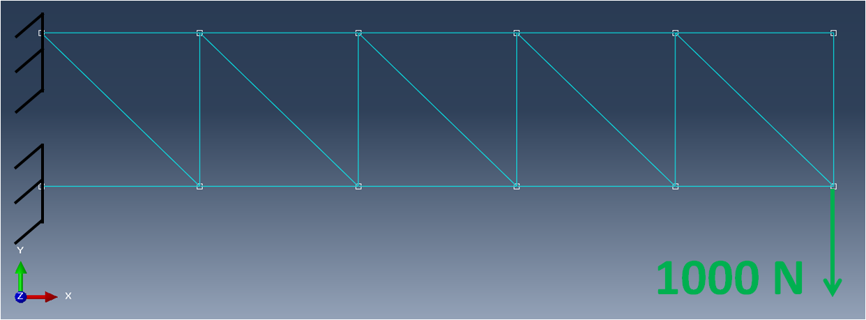
As you can see from the picture, the nodes are located at trusses intersections. Each truss is $ 1 m $ long and has an area of $ 40 mm^2 $ . A linear elastic material is applied with $ E = 200 GPa $ and $ \nu = 0.33 $ . The far left nodes are clamped while a vertical load of $ 1000 N $ is applied on the bottom right node.
This case is then solved as a linear static resolution.
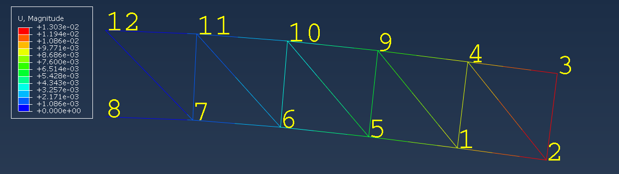
And the following figure gives an overview of the truss assembly displacements, as well as the node numbers.
To reproduce this simulation on your own, you need:
- at least the free version of the SesamX software installed,
- the truss assembly mesh (in Abaqus format),
- and the SesamX input cards (defining the element properties, the loading and so on).
If you are looking to extend this example, you can get help from the SesamX documentation.
Conclusion
I hope this article has provided you a better understanding of the truss finite element. If you are looking for more information, do not hesitate to send me and email.
Did you like this content?
Register to our newsletter and get notified of new articles