SesamX input file step by step guide
Introduction
This tutorial showcases how to write consistent SesamX input files from a beginner point of view. Together, we will write a complete input file setting up a simple shell model, and running a linear static resolution under a membrane solicitation. Along the way we will also discuss some Sesamx basic features (data persistence, units management, …).

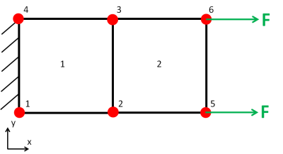
The model studied is made of 6 nodes and 2 quad shell elements. The material applied is linear elastic.
You can find all the relevant data related to this tutorial at the end of this page.
Data cards philosophy
First, let's talk about writing proper SesamX input file.
The major SesamX design philosophy is to follow an object paradigm. A SesamX model is made of objects (loads, constraints, solutions, …) that you can manipulate. you can think of these objects as data containers. You can operate on these containers through functions. Eventually, an input file is made of function calls following one another.
Under a function, the data is organized as a tree, as can be seen from the following example:
CREATE-LOAD
  NAME: MY_LOAD
  MODEL: MY_MODEL
  CONCENTRATED
    FORCE: 10000.,0.,0.
    MOMENT: 0.,0.,0.
    ON-NODES-FROM: LOAD_SELE
  # This is a comment line
This card is essentially a CREATE-LOAD function. As its name states, it creates a load named MY_LOAD which belongs to the model MY_MODEL. To do so, it assigns a concentrated force vector on each node of the selection LOAD_SELE. We define some basic vocabulary:
CREATE-LOADis a function. A function is always found at the root level of the input file. A function cannot be nested into another function.CONCENTRATEDis a branch. A branch is always found under a function or under another branch and may not be unique. It details how the function must behave.- Finally
NAME: MY_LOADis a keyword with an assigned value. A keyword may be found under a branch or directly under a function.
There is no order to observe in the data cards as long as the hierarchy of functions, branches and keywords is respected. However, the input file is sensitive to indentation (space indent). In fact through the indentation, SesamX knows how the data is structured.
You can add comment lines to your input file. A comment line must start with a #, as shown in the previous example.
Eventually, while downloading SesamX you will find into the installation package a Notepad++ user language cleverly highlighting the SesamX input file.
Units management
SesamX handles units natively. You do not need to feed consistent data. A partial recap of the default units used is provided below.
| Physical quantity | Unit |
|---|---|
| Length | $m$ |
| Thickness | $mm$ |
| Translation | $mm$ |
| Rotation | $°$ |
| Modulus | $GPa$ |
| Density | $Kg/m^3$ |
| Stress | $MPa$ |
| Strain | $\%$ |
| Translational stiffness | $N/m$ |
| Rotational stiffness | $Nm/rad$ |
| Force | $N$ |
| Moment | $Nm$ |
| Time | $s$ |
Of course, you are free to define your own units. To make things easier, SesamX always outputs a summary of the units used while running an input file.
Allocate a database
First of all, a database file must be created. This file will then contain all the data about the model we are about to create (the mesh, the loads, the solutions and so on). To define a database we simply need to use the SET-DATABASE function:
SET-DATABASE
  PATH="..\output\100_db.h5"
During this tutorial, we are only going to manipulate this database through SesamX. However, you can notice that the database file format is HDF5. It is a open format which allows you to manipulate the model data independently of SesamX (with a custom script for instance).
Create a new model
The next step is to create a model, using the following cards:
CREATE-MODEL
  NAME: MY_MODEL
You can create multiple models in the same SesamX database, each with a different name.
Create a mesh
Next come the mesh definition.
ADD-MESH
  MODEL: MY_MODEL
  NODES
    - ID: 1  POINT: 0.,0.,0.
    - ID: 2  POINT: 100.,0.,0.
    - ID: 3  POINT: 100.,100.,0.
    - ID: 4  POINT: 0.,100.,0.
    - ID: 5  POINT: 200.,0.,0.
    - ID: 6  POINT: 200.,100.,0.

  ELEMENTS
    SHAPE: QD4
    - ID: 1  NODES: 1,2,3,4
    - ID: 2  NODES: 2,5,6,3
Here we define 6 nodes and 2 elements on the model MY_MODEL. Nodes and elements are provided through a listing of coordinates and connectivities. An alternative syntax allows to import an Abaqus .inp mesh or a Salome .med file.
Create selections
A selection is composed of nodes and elements. Here we are defining 3 selections:
ALL_SELEwith all the nodes and elements of the model,LOAD_SELEwith the nodes on which we will apply the loading,BOUND_SELEwith the nodes on which we will apply the boundary condition.
CREATE-SELECTION
  MODEL: MY_MODEL
  NAME: ALL_SELE
  NODES-LIST
    IDS: 1,2,3,4,5,6
  ELEMENTS-LIST
    IDS: 1,2

CREATE-SELECTION
  MODEL: MY_MODEL
  NAME: LOAD_SELE
  NODES-LIST
    IDS: 5,6

CREATE-SELECTION
  MODEL: MY_MODEL
  NAME: BOUND_SELE
  NODES-LIST
    IDS: 1,4
Create a material and element properties
To define a linear isotropic material we need the Young's modulus and the Poisson's ratio. We also provide the density to complete the material definition.
CREATE-MATERIAL
  MODEL: MY_MODEL
  NAME: MY_MAT
  ELASTIC-ISOTROPIC
    E: 200.
    NU: 0.33
    DENSITY: 1.0E5
To define the shell property only the thickness of the element is needed.
SET-PROPERTIES
  MODEL: MY_MODEL
  SHELL-MITC
    NAME: PROP1
    TH: 1.0
    MATERIAL: MY_MAT
    ON-ELEMENTS-FROM: ALL_SELE
You can notice how to specify the elements on which to apply the property. ON-ELEMENTS-FROM: ALL_SELE means we want to select the elements from the selection ALL_SELE.
Create loading and boundary conditions
In this example we are assigning a $10000 N$ nodal force along the $x$ direction on the nodes 5 and 6 belonging to the selection LOAD_SELE. We use the CREATE-LOAD function.
CREATE-LOAD
  NAME: MY_LOAD
  MODEL: MY_MODEL
  CONCENTRATED
    FORCE: 10000.,0.,0.
    MOMENT: 0.,0.,0.
    ON-NODES-FROM: LOAD_SELE
And we are clamping the nodes 1 and 4 belonging to the selection BOUND_SELE. We use the CREATE-CONSTRAINT function.
CREATE-CONSTRAINT
  MODEL: MY_MODEL
  NAME: MY_CONST
  DISPLACEMENT-SPC
    TX: 0.
    TY: 0.
    TZ: 0.
    RX: 0.
    RY: 0.
    RZ: 0.
    ON-NODES-FROM: BOUND_SELE
You can define multiple loads and constraints in your model as long as you provide a distinct name for each.
Run a linear static resolution
At this point, we have completed the model definition and we have defined all the physical data necessary to run a static resolution. Which we can do with the following card.
SOLVE
  NAME: MY_SOL
  MODEL: MY_MODEL
  GEOM-NL: NO

  STEPS
    STATIC-STRESS
      NAME: LOADING
      NB-LEVELS: 1
      LOADS
        - NAME: MY_LOAD  AMPLITUDE-FUNCTION: "t"
      CONSTRAINTS
        - NAME: MY_CONST  AMPLITUDE-FUNCTION: "t"
We have to provide the load case and the boundary condition as well as parameters useful for the resolution. By default, the SOLVE function will look for singularities among the degrees of freedom, and fix them in order to solve the problem.
This function will result in the creation of a solution object that contains the displacements at the nodes. This solution object is then the entry point to the post-processing.
Post process the results
Visualization of data is performed through the OUTPUT-IMAGE function, in which we specify the information needed. The path to the generated image file as well as the name of the model is required. Then we have to select on which SesamX object we want to output some data, and finally what kind of data is desired.
Let's take the following example:
OUTPUT-IMAGE
  PATH: "..\output\100_IMG_MY_MODEL.h5"
  MODEL: MY_MODEL

  SOLUTION
    NAME: MY_SOL

    STEP
      NAME: LOADING
      TRANSLATION
        FIELD-NAME: MY_TRANS
      STRESS
        FIELD-NAME: MY_STRESS
Here we ask SesamX to produce an image file containing the translation field (named MY_TRANSin the image file) and the stress field (named MY_STRESSin the image file) from the solution MY_SOL.
The output file format is also HDF5.
Conclusion
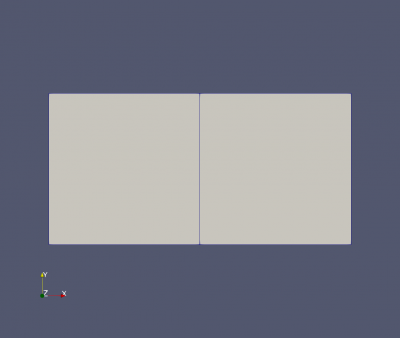
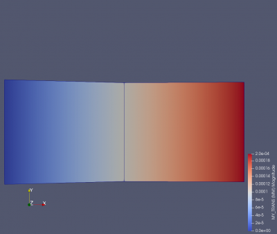
You can refer to the documentation in order to submit this input file, and visualize the results. You should visualize the following model and deformation.


From now on, you should feel comfortable reading the SesamX user manual to strengthen your skills. You can also consult our other tutorials.