This article aims at detailing how to derive an efficient triangular shell finite element, known as the MITC3 shell element(Mixed Interpolation of Tensorial Components). Most of the MITC3 element derivation is similar to that of the MITC4 element, already introduced in a previous article about the shell finite element. It is therefore not detailed again here. Instead, this article focuses on the specific features of the MITC3 element, such as the presence of an internal node, and how it is embedded into the element formulation using static condensation (also known as Guyan reduction).
Finally I will conclude this article with an example of an hyperboloid-like model, made of triangular shell elements, and simulated using the SesamX finite element analysis software (implementing the element presented here).
Quick remark on notations
Before starting, let’s define some notations that are used through this article:
vectors are denoted with an underline $ \underline{u} $ and tensors with a double underline $ \underline{\underline{\varepsilon}} $ ,
matrices are represented with brackets, as well as vector and tensor components $ \lbrack \ \rbrack $ ,
Einstein summation convention is used on repeated indices,
partial derivatives are denoted with the comma notation $ u_{,x} $ ,
infinitesimal strain and stress tensors are represented in column matrix notation $ \lbrack \varepsilon \rbrack = \begin{bmatrix} \varepsilon_{11} \\ \varepsilon_{22} \\ \varepsilon_{33} \\ 2 \varepsilon_{12} \\ 2 \varepsilon_{23} \\ 2 \varepsilon_{13} \end{bmatrix} $ and $ \lbrack \sigma \rbrack = \begin{bmatrix} \sigma_{11} \\ \sigma_{22} \\ \sigma_{33} \\ \sigma_{12} \\ \sigma_{23} \\ \sigma_{13} \end{bmatrix} $ , where $ \lbrack \varepsilon \rbrack $ represents the engineering strains.
Introducing the triangular shell finite element
When meshing a complex shell surface using automatic mesher, quadrangular and triangular elements are required. Hence, to be practical, a finite element solver must provide both elements and they must be reliable.
A great amount of work has been dedicated to quadrangular shell element, which have led to an improved MITC4 element, one of the most practical and efficient shell element. Triangular shell elements have not gathered the same focus. Nevertheless, a similar Mixed Interpolation of Tensorial Components (MITC) can be applied to the triangular element. And recent developments resulted in one of the best triangular shell element so far: the MITC3 element that we are discussing here. You can find every detail about this element in the following papers:
Lee PS, Bathe KJ. Development of MITC isotropic triangular shell finite elements: original paper about the MITC technique applied to triangular element.
Lee Y, Lee PS, Bathe KJ. The MITC3+ shell element and its performance: recent paper exposing new improvement to the MITC3 element.
The MITC3 element is conceptually similar to the MITC4 element. However the main difference between them is that the MITC3 element use an additional internal node in order to improve its bending behavior. This additional node does not come from the mesh and is automatically taken into account by the MITC3 formulation.
As for the MITC4, the MITC3 relies on the same shell characteristics and each of the following quantities are available at the nodes:
the position of the node $ \underline{X^I} $ ,
the thickness at the node $ h^I $ ,
the shell director vector at the node $ \underline{v^I} $ ,
the displacement vector at the node $ \underline{u^I} $ ,
and the rotation vector at the node $ \underline{\theta^I} $ .
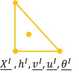
The director vector and thickness at the internal node are simply assumed to be the mean values from the corner nodes.
MITC3 shell element assumptions
The MITC3 element relies on assumptions that make it relevant to modelize shell structure. Even though these assumptions are similar to the MITC4 assumptions, they are specific to the MITC3 because of the internal node.
Stress assumption
The stress assumption mentioned for the MITC4 element still holds for the MITC3. In fact, it is the classical stress assumption made for shell and it does not depend on the shape of the element. We assume:
$$ \boxed{\sigma_{33} = 0} \tag{1} $$
We recall that in the case of the MITC element, the “3” direction is collinear to the director vector at each point of the shell mid-surface.
Kinematic assumption
The kinematic assumptions must take into account the presence of the internal node. Therefore, these kinematic assumptions are specific to the MITC3 element.
Position vector
Using the parametric coordinates, we have for the position of every point in the element:
$$ \underline{X}(r,s,t) = \underline{X_0}(r,s) + \cfrac{t}{2} h(r,s) \underline{v}(r,s) $$
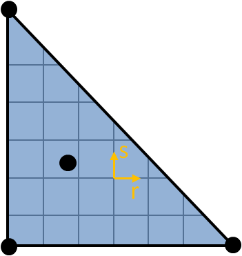
In the case of the MITC3, the parametric coordinates are showcased in the following figure.
However, the MITC3 does not rely only on the classical 2D shape functions of the triangular element. Indeed, the full expression of the position from the parametric coordinates is given by:
$$ \boxed{\underline{X}(r,s,t) = \displaystyle\sum_{I=1}^3 N^I(r,s)\underline{X^I} + \displaystyle\sum_{I=1}^4 \cfrac{t}{2} F^I(r,s)h^I \underline{v}^I} \tag{2} $$
Where the $ N^I $ shape functions are the classical 2D shape functions:
$$ \begin{cases} N^1(r,s) = 1-r-s \\ N^2(r,s) = r \\ N^3(r,s) = s \\ \end{cases} $$
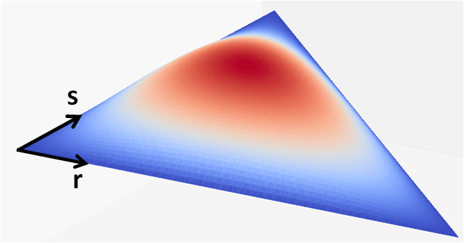
And the $ F^1, F^2, F^3 $ shape functions are the classical 2D shape functions, augmented with the cubic bubble shape function $ F^4 $ :
$$ \begin{cases} F^4(r,s) = 27rs(1-r-s) \\ F^1(r,s) = N^1(r,s) - \cfrac{1}{3}F^4(r,s) \\ F^2(r,s) = N^2(r,s) - \cfrac{1}{3}F^4(r,s) \\ F^3(r,s) = N^3(r,s) - \cfrac{1}{3}F^4(r,s) \\ \end{cases} $$
This cubic bubble function is associated with the internal node located at the center of the element ($ r = \cfrac{1}{3}, s = \cfrac{1}{3} $ ), and it is such that it vanishes on the element edges.
We note from the formula given in (2) that the internal node appears only in the second part of the relation.
Displacement vector
Next we express the displacement vector at each point inside the shell, relative to its parametric coordinates:
$$ \underline{u}(r,s,t) = \underline{u_0}(r,s) + \cfrac{t}{2} h(r,s) (\underline{\theta}(r,s) \times \underline{v}(r,s)) $$
Applying the interpolation from the nodes values, we have finally:
$$ \boxed{\underline{u}(r,s,t) = \displaystyle\sum_{I=1}^3 N^I(r,s)\underline{u^I} + \displaystyle\sum_{I=1}^4 \cfrac{t}{2} F^I(r,s) h^I (\underline{\theta^I} \times \underline{v^I})} \tag{3} $$
Obviously, the internal node appears only through its rotation degrees of freedom $ \underline{\theta^4} $ .
It is important to remark here that these new degrees of freedom are treated the same as the other degrees of freedom. Hence, they do not add complexity when deriving the stiffness matrix.
However, they are peculiar because they are not attached to a node belonging to the mesh. Therefore, these internal degrees of freedom are not shared between adjacent elements, which can have useful consequences when assembling the stiffness matrix (as discussed a bit further).
On a kinematic point of view, these additional degrees of freedom enrich the element displacement capabilities. In fact, they improve the element bending behavior.
Basis and coordinate systems
The basis and coordinate systems used here are the same as those introduced in the shell finite element article.
MITC3 shell element derivation
Next, the classical MITC procedure is applied to derive the element strain components. These strain components are computed at specific locations (known as tying points) inside the element, and they are interpolated to provide the strain values anywhere inside the element (for instance at Gauss points).
If you are looking for the full MITC procedure employed for the MITC3 element, you can refer to [2].
Applying the classical finite element method we can derive the shell element stiffness matrix.
MITC3 shell element stiffness matrix
The element stiffness matrix is obtained through the expression of the virtual work. Denoting the virtual strains as $ \lbrack \overline{\varepsilon} \rbrack $ we have for the virtual work over the element volume:
$$ \overline{W} = \iiint_V \lbrack \overline{\varepsilon} \rbrack^T \lbrack \sigma \rbrack dV $$
As for the MITC4 element, applying the change of variable from the local Cartesian coordinate system to the parametric coordinate system leads to:
$$ \overline{W} = \iiint_V \lbrack \overline{\varepsilon} \rbrack^T \lbrack D \rbrack \lbrack \varepsilon \rbrack |\underline{g_t} \cdot (\underline{g_r} \times \underline{g_s})| drdsdt $$
Where now $ V $ denotes the element volume in the parametric coordinate system.
We need to apply the 7-point Gauss integration to integrate exactly on the plane defined by $ r $ and $ s $ , because of the cubic bubble function we used to express the displacement. Besides, this integrand depends arbitrarily on $ t $ and therefore we cannot “pre-integrate” through the thickness. We use then a 2-point Gauss integration on $ t $ that has proven to be accurate enough for most applications.
Finally we can write:
$$ \boxed{ \overline{W} = \displaystyle\sum_{i=1}^{14} w_i \underbrace{\lbrack \overline{\varepsilon} \rbrack^T \lbrack D \rbrack \lbrack \varepsilon \rbrack |\underline{g_t} \cdot (\underline{g_r} \times \underline{g_s})|} _{\text{evaluated at the point }r_i, s_i, t_i} } \tag{4} $$
Where $ w_i, r_i, s_i, t_i $ are given in the following table (source G. R. Cowper):
| Point | $ w_i $ | $ r_i $ | $ s_i $ | $ t_i $ |
|---|---|---|---|---|
| 1 | 0.0629695902724 | 0.1012865073235 | 0.1012865073235 | -0.5773502691896 |
| 2 | 0.0629695902724 | 0.7974269853531 | 0.1012865073235 | -0.5773502691896 |
| 3 | 0.0629695902724 | 0.1012865073235 | 0.7974269853531 | -0.5773502691896 |
| 4 | 0.0661970763943 | 0.4701420641051 | 0.0597158717898 | -0.5773502691896 |
| 5 | 0.0661970763943 | 0.4701420641051 | 0.4701420641051 | -0.5773502691896 |
| 6 | 0.0661970763943 | 0.0597158717898 | 0.4701420641051 | -0.5773502691896 |
| 7 | 0.1125 | 0.3333333333333 | 0.3333333333333 | -0.5773502691896 |
| 8 | 0.0629695902724 | 0.1012865073235 | 0.1012865073235 | 0.5773502691896 |
| 9 | 0.0629695902724 | 0.7974269853531 | 0.1012865073235 | 0.5773502691896 |
| 10 | 0.0629695902724 | 0.1012865073235 | 0.7974269853531 | 0.5773502691896 |
| 11 | 0.0661970763943 | 0.4701420641051 | 0.0597158717898 | 0.5773502691896 |
| 12 | 0.0661970763943 | 0.4701420641051 | 0.4701420641051 | 0.5773502691896 |
| 13 | 0.0661970763943 | 0.0597158717898 | 0.4701420641051 | 0.5773502691896 |
| 14 | 0.1125 | 0.3333333333333 | 0.3333333333333 | 0.5773502691896 |
Static condensation of the stiffness matrix
The MITC3 stiffness matrix is expressed on the degrees of freedom at the 3 corner nodes plus the internal node. This matrix has $ \underbrace{3 \times 6}_{\text{corner nodes}} + \underbrace{3}_{\text{internal node}} = 21$ rows and columns.
However, under certain circumstances, we can factorize this stiffness matrix to express it only on the degrees of freedom at the corner nodes. This factorization is known as the static condensation, and is detailed here.
Regrouping the external degrees of freedom on one hand, and the internal ones on the other hand, we can write the element stiffness matrix as follows:
$$ \lbrack K_{elem} \rbrack = \begin{bmatrix} \lbrack k_{ee} \rbrack & \lbrack k_{ei} \rbrack \\ \lbrack k_{ei} \rbrack ^T & \lbrack k_{ii} \rbrack \\ \end{bmatrix} $$
Where:
$ \lbrack k_{ee} \rbrack $ relates the external dofs to the external dofs (size $ 18 \times 18 $ ),
$ \lbrack k_{ii} \rbrack $ relates the internal dofs to the internal dofs (size $ 3 \times 3 $ ),
$ \lbrack k_{ei} \rbrack $ relates the external dofs to the internal dofs (size $ 18 \times 3 $ ).
In the same manner, we can write the element displacement and force column matrices (both have 21 components) as:
$$ \lbrack X_{elem} \rbrack = \begin{bmatrix} \lbrack X_e \rbrack \\ \lbrack X_i\rbrack \\ \end{bmatrix} $$
and
$$ \lbrack F_{elem} \rbrack = \begin{bmatrix} \lbrack F_e \rbrack \\ \lbrack F_i\rbrack \\ \end{bmatrix} $$
Let’s assume we are computing the stiffness matrix in order to perform a static linear resolution. For a given displacement vector on the element, the reaction force vector is given by:
$$ \lbrack F_{elem} \rbrack = \lbrack K_{elem} \rbrack \lbrack X_{elem} \rbrack $$
And after expanding, we have the following relations:
$$ \boxed{ \begin{cases} \lbrack F_e \rbrack = \lbrack k_{ee} \rbrack \lbrack X_e \rbrack + \lbrack k_{ei} \rbrack \lbrack X_i \rbrack \\ \lbrack F_i \rbrack = \lbrack k_{ei} \rbrack^T \lbrack X_e \rbrack + \lbrack k_{ii} \rbrack \lbrack X_i \rbrack \end{cases} }\tag{5} $$
However, as mentioned previously, the internal degrees of freedom are not attached to a node belonging to the mesh. Hence, the internal dofs do not carry any load. This translates to:
$$ \lbrack F_i \rbrack = \lbrack 0 \rbrack $$
Solving the second relation of (5) for $ \lbrack X_{i} \rbrack $ gives:
$$ \lbrack X_{i} \rbrack = - \lbrack k_{ii} \rbrack^{-1} \lbrack k_{ei} \rbrack^T \lbrack X_e \rbrack $$
And inserting this result in the first relation of (5) yields:
$$ \boxed{ \lbrack F_e \rbrack = \underbrace{\lbrack k_{ee} \rbrack \lbrack X_e \rbrack - \lbrack k_{ei} \rbrack \lbrack k_{ii} \rbrack^{-1} \lbrack k_{ei} \rbrack^T} _{\lbrack K_{elem}' \rbrack} \lbrack X_e \rbrack } $$
Where $ \lbrack X_{i} \rbrack $ does no longer appear. We finally arrive at the expression of the condensed stiffness matrix $ \lbrack K_{elem}' \rbrack $ relating only the external degrees of freedom.
The main advantage of this condensation is that it can be performed on the element level before assembling the whole stiffness matrix. Whether we apply this condensation or not will lead to the same displacement result in the end.
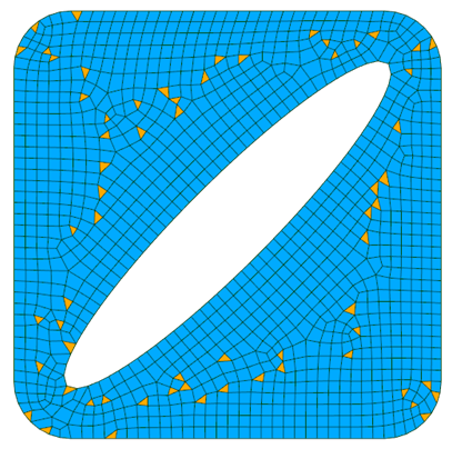
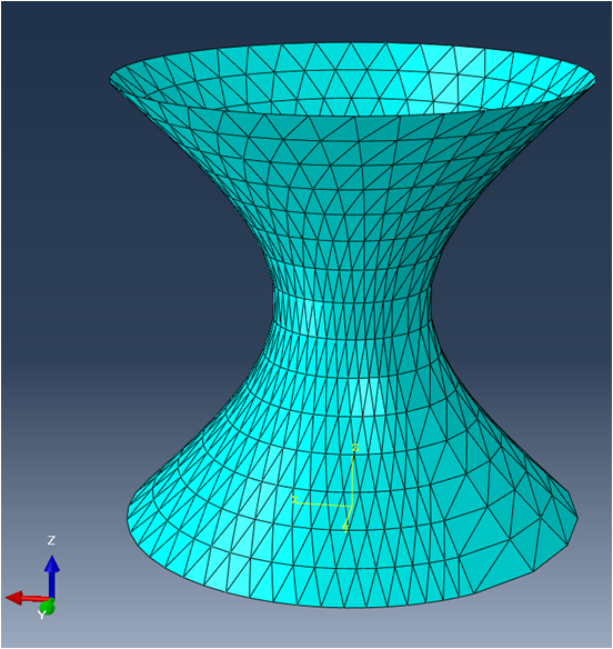
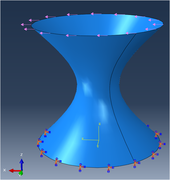
Example of a simple structure using shell elements
As an example, the following hyperboloid-like model is set up and simulated with the SesamX finite element software.
 |
 |
|---|---|
The mesh is voluntarily distorted and curved. This mesh can be qualified as a bad mesh, however it is useful to showcase the robustness of the MITC3 shell element.
A linear elastic material is applied with $ E = 200 GPa $ and $ \nu = 0.33 $ and a thickness of $ 80 mm $ is applied on all the elements. The circle at $ Z = 0 $ is clamped while a uniformly distributed load along $ X $ is applied at the top circle of the hyperboloid.
This case is then solved with a linear static resolution.
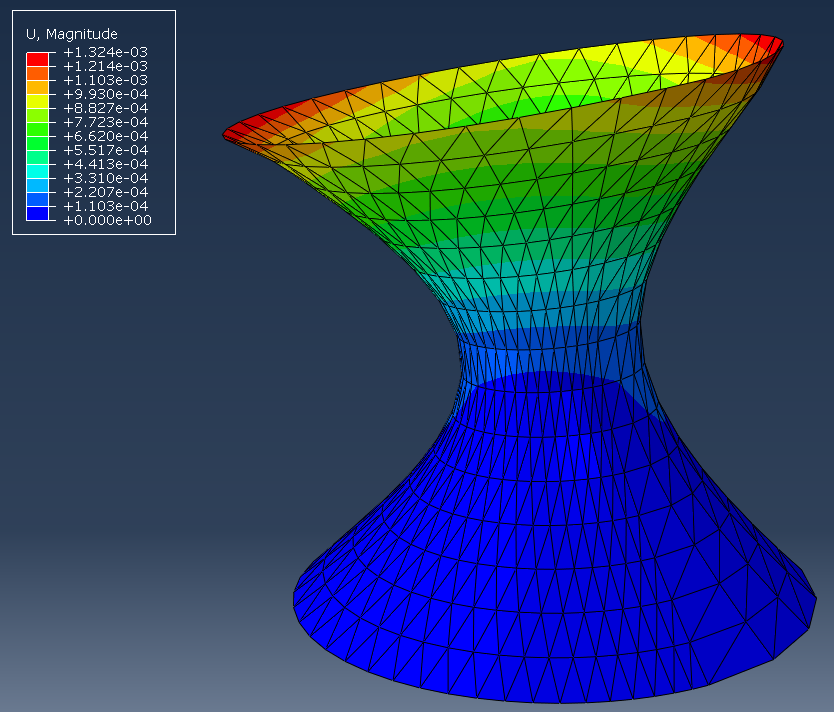
And the following figure illustrates the displacement of the model.
To reproduce this simulation on your own, you need:
- at least the free version of the SesamX software installed,
- the shell model mesh (in Abaqus format),
- and the SesamX input cards (defining the element properties, the loading and so on).
If you are looking to extend this example, you can get help from the SesamX documentation.
Conclusion
I hope this article has provided you a better understanding of the shell finite element. If you are looking for more information, do not hesitate to send me and email.
Did you like this content?
Register to our newsletter and get notified of new articles