The shell finite element explained

The development of an efficient shell element has gathered a lot of work since the beginning of structural finite element history. For multiple reasons, developing an effective shell element is not an easy task, and we will cover some of these reasons through this article. Multiple shell elements are available in the literature, and they are still being improved as time goes on. For this article I have decided to introduce the MITC shell element (Mixed Interpolation of Tensorial Components) because it recently received new improvements making it one of the most practical and efficient shell element. After detailing the various assumptions and how they work together, I will explain how to derive the shell element stiffness matrix. Finally, I will conclude this article with an example of an hyperboloid-like model simulated using the SesamX finite element analysis software (implementing the element presented here).

There are 2 main kinds of shell element depending on their underlying geometry: quadrangular and triangular. In this article I will focus on the MITC4 element (quadrangular) because it is the most widespread among the MITC shell family.

Relevant papers about the MITC4 shell finite element

This article is mainly inspired from the following papers about the MITC4 element. They are great resources to consult if you are looking for deeper information about this element.

1. Dvorkin EN, Bathe KJ. A continuum mechanics based four-node shell element for general nonlinear analysis: original paper about the MITC4 element. It introduces the concept of mixed interpolation of tensorial components, and how it improves the transverse shear behavior of the element.

2. Ko Y, Lee PS, Bathe KJ. A new MITC4+ shell element: recent paper exposing new improvements about the MITC4 element membrane behavior.

3. Ko Y, Lee PS, Bathe KJ. A new 4-node MITC element for analysis of two dimensional solids and its application in shell analyses: other improvements about the MITC4 element membrane behavior.

4. Ko Y, Lee Y, Lee PS, Bathe KJ. Performance of the MITC3+ and MITC4+ shell elements in widely-used benchmark problems: comparison of the improved MITC4 element against other well known shell elements (including Abaqus S4 element).

Quick remark on notations

Before starting, let’s define some notations that are used through this article:

• vectors are denoted with an underline $\underline{u}$ and tensors with a double underline $\underline{\underline{\varepsilon}}$ ,

• matrices are represented with brackets, as well as vector and tensor components $\lbrack \ \rbrack$ ,

• Einstein summation convention is used on repeated indices,

• partial derivatives are denoted with the comma notation $u_{,x}$ ,

• infinitesimal strain and stress tensors are represented in column matrix notation $\lbrack \varepsilon \rbrack = \begin{bmatrix} \varepsilon_{11} \\ \varepsilon_{22} \\ \varepsilon_{33} \\ 2 \varepsilon_{12} \\ 2 \varepsilon_{23} \\ 2 \varepsilon_{13} \end{bmatrix}$ and $\lbrack \sigma \rbrack = \begin{bmatrix} \sigma_{11} \\ \sigma_{22} \\ \sigma_{33} \\ \sigma_{12} \\ \sigma_{23} \\ \sigma_{13} \end{bmatrix}$ , where $\lbrack \varepsilon \rbrack$ represents the engineering strains.

Introducing the shell element

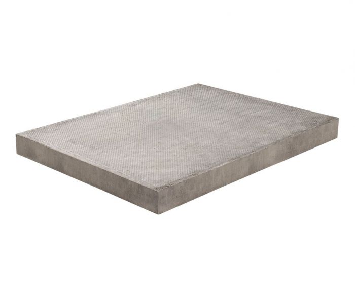
The shell element is intended to analyze thin structures undergoing forces and moments in any direction. The structure can be flat or curved but it should have one dimension smaller than the other 2. For instance, it is the perfect element to analyze a slab or an aircraft fuselage.

Slab	Aircraft fuselage

To fully define the shell geometry, the element needs the following 3 characteristics:

• The mid-surface geometry,

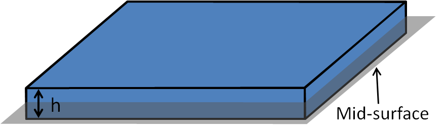
• The thickness at each point of the mid-surface: $h$ ,

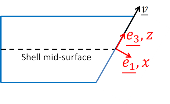
• The director vector at each point of the mid-surface: $\underline{v}$

The mid-surface and thickness are what comes naturally in mind when thinking about shells.

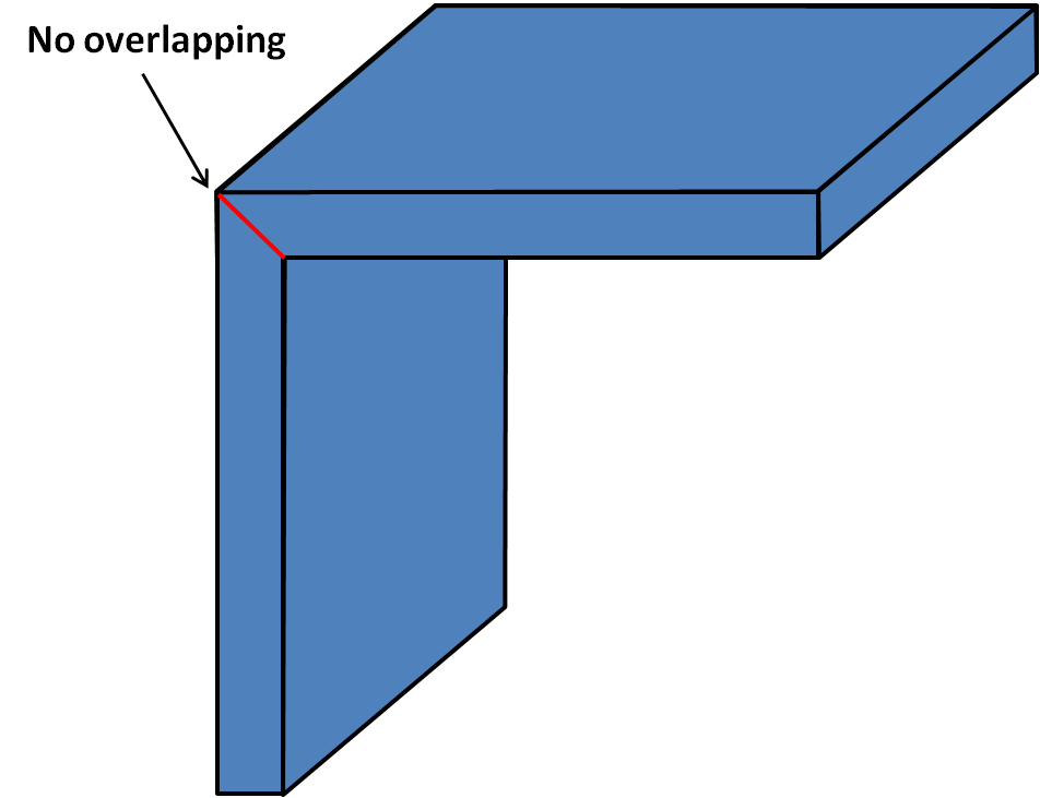
The director vector is a specific MITC feature. It allows to control how the “cross section” is tilted relative to the mid-surface.

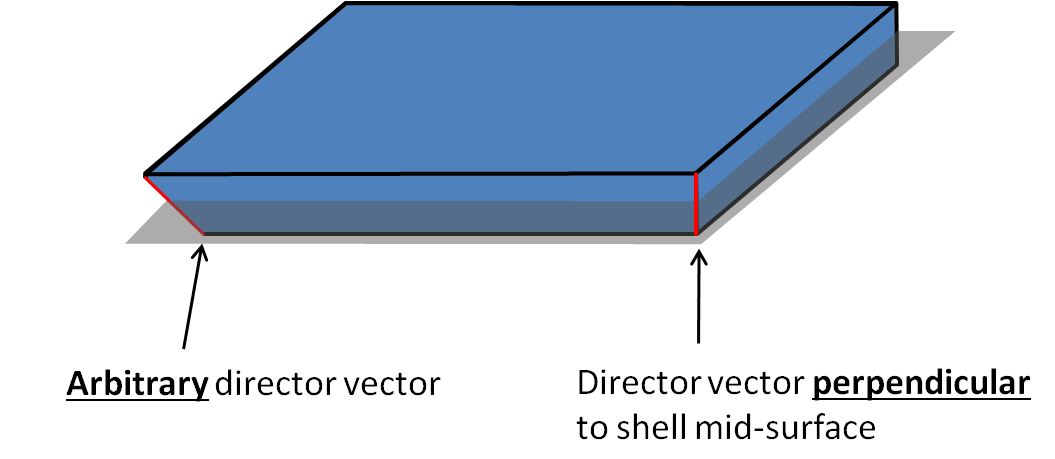
Theses features make it possible to modelize shells with varying thickness along the mid-surface, as well as arbitrary shells connections.

Varying shell thickness	Shell connection

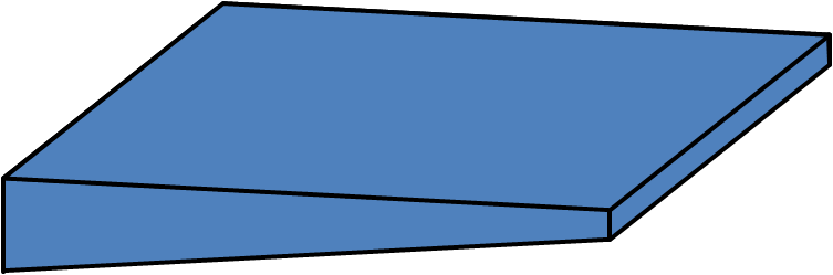
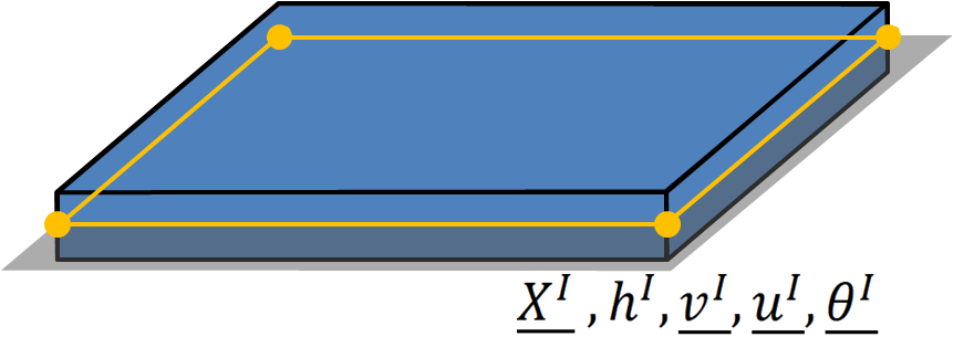
Furthermore, this element is not restricted to flat shell and can also represent curved geometries. The element is meshed on the mid-surface using 4 nodes. At each node $I$ the following quantities are available:

• the position of the node $\underline{X^I}$ ,

• the thickness at the node $h^I$ ,

• the shell director vector at the node $\underline{v^I}$ ,

• the displacement vector at the node $\underline{u^I}$ ,

• and the rotation vector at the node $\underline{\theta^I}$ .

MITC4 shell element assumptions

In essence, the shell element is a simplification of a more complex 3D structure. When designing such an element, the aim is to decrease the computational cost, while making relevant assumptions on how the element behaves. The main kinematic assumptions underlying the MITC element are given here with some explanations.

Stress assumption

As the shell must be able to sustain transverse and plane loading, the stress state must allow for transverse shear stress, as well as in plane stress. It is then sufficient to enforce:

This is the classical stress assumption made for shell elements when the “3” direction is normal to the mid-surface. However, in the case of the MITC element, the “3” direction is collinear to the director vector at each point of the shell mid-surface (basis and coordinate systems are detailed further ahead in this article).

Kinematic assumption

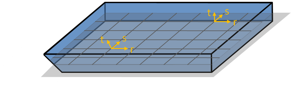
Before detailing the kinematic assumption, we need to define a convenient parametric coordinate system on the shell.

Parametric coordinates system and position vector

We rely on the position vector to define the parametric system. Without providing more details, the first 2 coordinates $r$ and $s$ can be any of the mid-surface curvilinear coordinates. The last coordinate $t$ is such that for a given $r$ and $s$ , $t$ evolves when we move along the director vector.

Using these parametric coordinates, we can describe the position of every point in the space:

Where $\underline{X_0}(r,s)$ describes the mid-surface position. To define clearly what $r$ and $s$ are, we need to detail further $\underline{X_0}(r,s)$ , $h(r,s)$ and $\underline{v}(r,s)$ .

Using the position of the nodes and the shape functions we have:

• $\underline{X_0}(r,s) = N^I(r,s)\underline{X^I}$
• $h(r,s) \underline{v}(r,s) = N^I(r,s)h^I \underline{v}^I$

Where the shape functions $N^I$ are:

Which yields the full expression of the position from the parametric coordinates:

Please note the following remarks:

• for $t = 0$ the domain $r, s \in [-1, 1]$ describes the shell mid-surface,

• $t$ moving from -1 to 1 corresponds to a point moving from the inferior face to the superior face of the shell,

• the full product $h(r,s) \underline{v}(r,s)$ is linearly interpolated from its values at the nodes (we want to stress that $h(r,s)$ and $\underline{v}(r,s)$ are not interpolated on their own but through their product),

• even though expression (3) is useful to define the parametric space, we use extensively expression (2) in the following for its conciseness.

Displacement vector

Next we express the displacement vector at each point inside the shell, relative to its parametric coordinates. We have:

Where:

• $\underline{u_0}(r,s)$ is the displacement vector on the shell mid-surface,

• $\underline{\theta}(r,s)$ is the rotation vector on the shell mid-surface.

We see from this formula that, for a given point on the mid-surface, the rotation vector $\underline{\theta}(r,s)$ describes simply the rotation of the director vector. Hence $\cfrac{t}{2} h(r,s) (\underline{\theta}(r,s) \times \underline{v}(r,s))$ is simply the displacement resulting from the director vector rotation.

However, this comes at a price. In general, if we seek to compute the rotation of a vector $\underline{v}$ under a given rotation vector $\underline{\theta}$ , we have to apply Rodrigues’ formula. This formula is non linear on $\underline{\theta}$ , but can be simplified to $\underline{\theta} \times \underline{v}$ if we assume that $\underline{\theta}$ is small (which is the case here).

As for the position vector, we relate the displacement inside the shell from the displacements and rotations at the nodes:

And we note again that the full term $h(r,s) (\underline{\theta}(r,s) \times \underline{v}(r,s))$ is interpolated at once from the values at the nodes. To make things easier, we can introduce the vector $\underline{\phi} = \underline{\theta} \times \underline{v}$ to finally write:

And after interpolation from the values at the nodes:

Basis and coordinate systems

Before going further, let’s define and summarize the different basis and coordinate systems that are used while deriving the stiffness matrix.

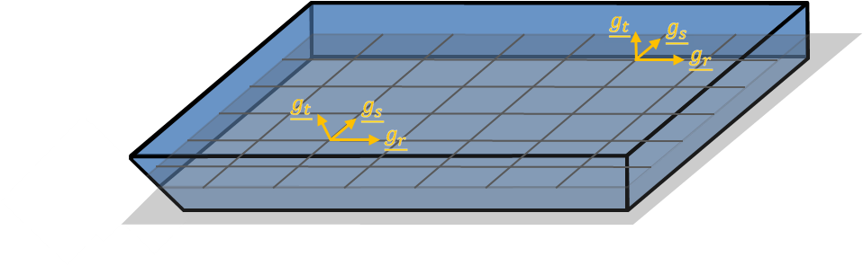
Covariant basis

We have defined previously the parametric coordinate system ($r$ , $s$ , $t$ ). It is time now to give the associated covariant basis. Using (2), this basis is defined as:

Remarks:

• $\underline{g_r}$ and $\underline{g_s}$ depend on $r$ , $s$ and $t$ while $\underline{g_t}$ depends only on $r$ and $s$ ,

• if the element has the same director vectors and thickness at the nodes, then $h \underline{v}$ is constant, and now $\underline{g_r}$ and $\underline{g_s}$ depend only on $r$ and $s$ ,

In a sense, the covariant basis “follows” the geometry of the element. Therefore, it is used to compute specific strains inside the element.

Contravariant basis

We will also use the contravariant basis associated with the previous covariant one. It is defined as follow:

This basis is used conjointly with the covariant basis to manipulate the strain tensor. In fact, it has the following properties: $\underline{g^i} \cdot \underline{g_j} = 0$ $\forall i,j \ i = \not j$ and $\underline{g^i} \cdot \underline{g_i} = 1$

Local basis and local Cartesian coordinate system

From the covariant basis, we also define a Cartesian local basis ($\underline{e_1}, \underline{e_2}, \underline{e_3}$ ) as follow:

And from this local basis, we define the local Cartesian coordinate system ($x$ , $y$ , $z$ ). We note that $\underline{e_3}$ is not perpendicular to the shell mid-surface but is aligned with $\underline{v}$ .

The local basis is used to express the stress strain relation for the shell. The stress assumption given in (1) applies in this basis. While the local Cartesian coordinate system is used to integrate the virtual work over the element volume.

Note that when $\underline{v}$ is not perpendicular to the mid-surface, the plane described by $\underline{e_1}$ and $\underline{e_2}$ is not on the mid-surface.

MITC4 shell element derivation

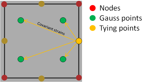
The biggest challenge regarding shell element design is to avoid shear and membrane locking, namely the tendency of the element to represent too rigidly shear and membrane motions. Multiple techniques have been employed to alleviate this issue, each having its pros and cons. Regarding the MITC, this issue is tackled without adding extra degree of freedom or instability to the element. Which makes it an efficient and conceptually simple shell element.

In fact, it relies on assuming specific transverse shear and membrane strains interpolation inside the element from strain values at tying points. And these points are specifically chosen to avoid locking. The fundamental assumption underlying the MITC element is the use of the covariant strain components to perform this interpolation. Roughly speaking, covariant strain components at the tying points are manipulated and inserted as covariant strain components at any point (for instance Gauss points). Hence the covariant / contravariant basis act as a hub connecting the strains from multiple points.

Applying the classical finite element method we can derive the shell element stiffness matrix.

Strain tensor

The strain tensor can be expressed in whatever basis we choose. To go on with the MITC procedure, we need to express the strains in the contravariant basis to get the covariant strain components. Then the tying procedure is applied on some of these terms to improve the element behavior.

Covariant strain tensor components

From definition, the covariant strains components are given by:

And it can be shown that:

Using (4) we can simplify further this expression:

Where the displacement and rotation vectors (through $\underline{\phi}$ ) appear more clearly. We note that $\widetilde{\varepsilon_{tt}} = 0$ because by definition $\underline{\phi}$ is perpendicular to $\underline{g_t}$ . The relations given here are valid for an arbitrary point inside the element. Next step is about modifying these terms from their values at the tying points.

Covariant transverse shear tying procedure

The procedure detailed here can be found in details in [1]. We are interested in reworking the terms $\widetilde{\varepsilon_{st}}$ and $\widetilde{\varepsilon_{rt}}$ that are responsible for transverse shear locking. The idea is to compute the term $\widetilde{\varepsilon_{st}}$ at the tying points C and D, and the term $\widetilde{\varepsilon_{rt}}$ at the tying points A and B (see picture below). Such that we have, $\widetilde{\varepsilon^A_{rt}}$ , $\widetilde{\varepsilon^B_{rt}}$ , $\widetilde{\varepsilon^C_{st}}$ and $\widetilde{\varepsilon^D_{st}}$ .

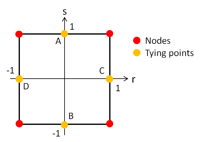
Note that these tying points are located on the mid-surface. Eventually, elsewhere in the element, $\widetilde{\varepsilon_{rt}}$ and $\widetilde{\varepsilon_{st}}$ are interpolated from the values at the tying points. Hence, for an arbitrary point located at $(r, s)$ we have:

Covariant membrane strain tying procedure

The full procedure can be found in [2] and [3]. It is more involved than the transverse shear procedure but quite similar. The idea is to rework the terms $\widetilde{\varepsilon_{rr}}$ , $\widetilde{\varepsilon_{ss}}$ and $\widetilde{\varepsilon_{rs}}$ such that membrane locking is suppressed by using specific tying points inside the element. As for the shear terms, it yields new relations for the terms $\widetilde{\varepsilon_{rr}}$ , $\widetilde{\varepsilon_{ss}}$ and $\widetilde{\varepsilon_{rs}}$ that linearly depend on strains at the tying points.

Summary

Once the tying procedure is completed, we can rewrite (9) using the covariant strains at the tying points. We then insert the displacement and rotation vectors interpolated from the nodes values (5). This yield the full expression of the covariant strain components that linearly depend on the degrees of freedom at the nodes.

The last step is then to project the covariant strain components into the local basis (8). Expressing the strain tensor in the contravariant basis on one hand and in the local basis on the other hand we have:

Which relates the covariant strain components to the local strain components:

Using the fact that $\widetilde{\varepsilon_{tt}} = 0$ and that $\underline{e_3}$ is collinear to $\underline{g_t}$ (hence $\underline{e_3} \cdot \underline{g^r} = \underline{e_3} \cdot \underline{g^s} = 0$ ) we can write the local strains in matrix representation (using engineering strains):

Stress tensor

To relate the stresses to the strains we need to apply Hooke’s law for linear elastic material.

Note that this material law is applied on strains and stresses expressed in the local basis (where $\underline{e_3}$ is not necessarily perpendicular to the mid-surface). Using assumption (1) on the right hand side, as well as the result we got in (10) on the left hand side, leads to a peculiar relation:

As for the truss element and beam element, this relation cannot hold. However using a similar explanation, we can find a way out. When making the kinematic assumption we were interested in the macroscopic behavior of the shell. Whereas the stress assumption relates more to a microscopic behavior. It turns out that even if $\varepsilon_{33}$ is not 0 (microscopic scale) its effect on the displacement (macroscopic scale) is negligible compared to what comes from the other terms. Of course, this explanation becomes questionable as the thickness of the shell increases.

We can therefore simplify this relation and write:

An finally we invert it and omit $\varepsilon_{33}$ and $\sigma_{33}$ to get the stresses from the strains:

Where the classical transverse shear correction factor $k = \cfrac{5}{6}$ was introduced.

MITC4 shell element stiffness matrix

The element stiffness matrix is obtained through the expression of the virtual work. Denoting the virtual strains as $\lbrack \overline{\varepsilon} \rbrack$ we have for the virtual work over the element volume:

Where $dV = dxdydz$ refers to the volume element in the local Cartesian coordinate system. However, the formula previously derived for the strains depends on the parametric coordinate system $(r, s, t)$ . We can relate this volume element to the parametric coordinates using the determinant of the Jacobian matrix:

It can be shown that the Jacobian matrix is directly given by the covariant vectors components expressed in the local basis:

Where $\lbrack g_i \rbrack$ represents the components of the vector $\underline{g_i}$ in the local basis.

Besides, it can be shown that as long as the $\lbrack g_i \rbrack$ are components of vectors in an orthonormal basis, we have:

Hence after expanding (11) we get the following expression:

Unlike classical shell or plate element, we cannot in general “pre-integrate” along $t$ this volume integral because the dependence on $t$ is arbitrary. We simply apply a numerical integration over $r$ , $s$ and $t$ . The 2 x 2 x 2 Gauss rule is enough to integrate exactly along $r$ and $s$ , and has proven to be accurate enough to integrate along $t$ for most applications (even though we cannot ensure an exact integration).

Remark: In the specific case where $h \underline{v}$ is constant over the element, we have seen that $\underline{g_r}$ and $\underline{g_s}$ no longer depend on $t$ . This makes it possible to integrate exactly along $t$ without requiring numerical integration.

Eventually, using (10), we can relate each of the terms obtained to the nodes displacements and rotations and recognize the expression of the stiffness matrix.

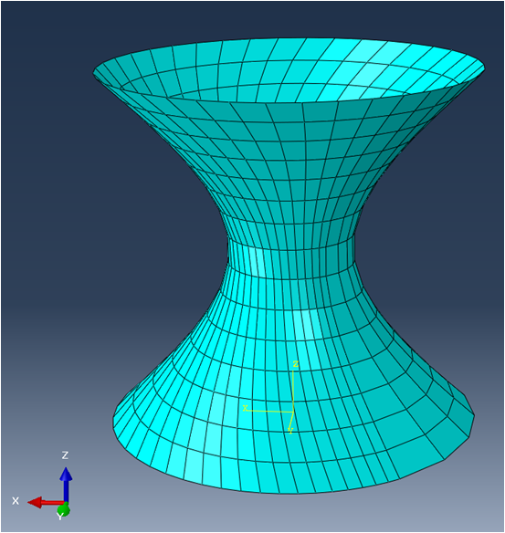
Example of a simple structure using shell elements

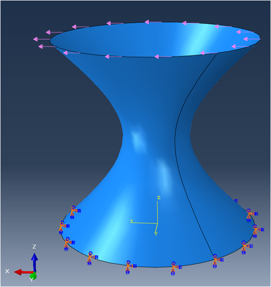
As an example, the following hyperboloid-like model is set up and simulated with the SesamX finite element software.

Mesh	Loading and boundary conditions

The mesh is voluntarily distorted and curved (the quads are not planar). This mesh can be qualified as a bad mesh, however it is useful to showcase the robustness of the MITC4 shell element.

A linear elastic material is applied with $E = 200 GPa$ and $\nu = 0.33$ and a thickness of $80 mm$ is applied on all the elements. The circle at $Z = 0$ is clamped while a uniformly distributed load along $X$ is applied at the top circle of the hyperboloid.

This case is then solved with a linear static resolution.

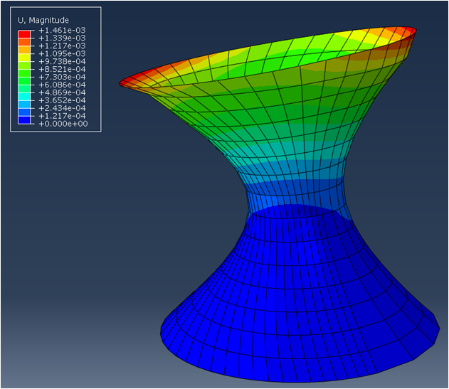
And the following figure illustrates the displacement of the model.

To reproduce this simulation on your own, you need:

• at least the free version of the SesamX software installed,
• the shell model mesh (in Abaqus format),
• and the SesamX input cards (defining the element properties, the loading and so on).

If you are looking to extend this example, you can get help from the SesamX documentation.

Conclusion

I hope this article has provided you a better understanding of the shell finite element. If you are looking for more information, do not hesitate to send me and email.