The importance of hardware for FEA

In this article, I am talking about hardware and finite element analysis. I will provide you the key concepts to understand why hardware is important for FEA. So that you can analyze on your own, what is the proper hardware requirement matching your finite element analysis needs.

Browsing the internet about the relation between finite element analysis and hardware can become tedious. A lot of information is available but it is quite often not obvious to get the general picture about the subject. Besides, nowadays the majority of finite element software vendors encourages us to use HPC cluster in order to perform efficient FEA. Furthermore, with the advent of cloud computing, it seems to become a one size fits all solution: every business (small, medium or large) can improve its cloud HPC cluster on demand, without the need to buy and maintain t he cluster’s hardware itself.

These kinds of statements should be taken with caution. HPC cloud cluster may be an appropriate solution for your business, but it can also become way more expensive than an equivalent physical solution. Most of the time, you are better off starting with physical and cheap solutions: it enables you to gain enough experience in order to judge if there are benefits to jump into HPC cloud cluster.

At SesamX, our mission is to provide affordable finite element analysis solution to our customers. But we also advise them about how to use finite element analysis intelligently. Do you always need expensive hardware to make FEA efficient? The answer is No. And I will explain why in this article.

First, I will explain why FEA is demanding on hardware, and what do we mean by efficient FEA. Then, we will see how FEA uses the main computer components (CPU, RAM and hard drive) and what are the differences between a workstation and a HPC cluster. Afterwards, I will share my thoughts and rules about choosing the right hardware depending on your FEA needs. And finally, I will present a case study showcasing what kind of performance gain SesamX can achieve on a workstation.

What makes FEA demanding on hardware?

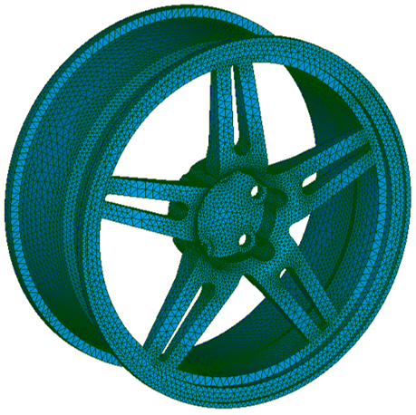
The essence of finite element analysis is to decompose a complex geometry into multiple elements. Each element forms a simple shape on which the physical equations of the problem are solved. Elements are connected to each other through nodes. And nodes carry the degrees of freedom of the system (also simply called dof): these degrees of freedom make the unknowns of the finite element problem to solve.

For instance:

• in mechanical analysis, the degrees of freedom are the displacements at the nodes in the 3D space (u, v, w).
• in thermal analysis, the degrees of freedom are the temperature at the nodes.

One obvious way to improve the precision of a model is to increase the number of elements and hence the number of degrees of freedom. But this has a cost:

• each element needs to be processed by the computer in order to set up the stiffness matrix,
• and as the number of degrees of freedom increases, it increases the size of the stiffness matrix.

For convenient reasons, we often only mention the number of degrees of freedom as the driving parameter for the model precision. We consider implicitly that the number of elements is directly linked to the number of degrees of freedom.

To conclude, the number of degrees of freedom is the major factor that makes FEA demanding on hardware: more degrees of freedom means more computations are required to solve the problem (i.e. to invert the stiffness matrix).

However, there is another important factor that we should not omit: the number of time steps (also called levels in SesamX). Usually, a non linear dynamic or even static resolution is split among multiple time steps. These time steps seek to discretize the time dependence of the problem.

And for each time step, there is one or more stiffness inversion required (depending on how the non linear resolution converges). Therefore, the number of time steps acts as a multiplying factor on the number of degrees of freedom.

Of course many other factors have an effect on the amount of computation. We can mention for instance the material behavior or contact conditions. However, these are secondary factors. And as we seek to get the general picture, we can conclude that the amount of computation needed to solve a finite element problem is proportional to the number of degrees of freedom times the number of time steps:

How hardware components relate to FEA software efficiency?

It is now time to define what an efficient FEA software really means. But first, we need to review how FEA software use the main hardware components available on a computer: the CPU (central processing unit), the RAM (random access memory) and the hard drive.

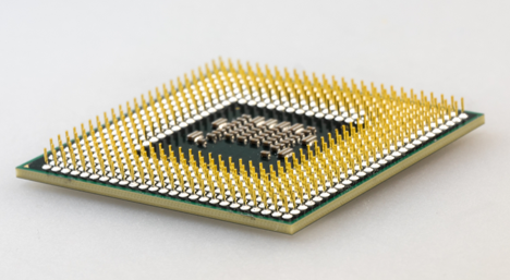
Let’s start with the CPU. The CPU is in charge of performing the various calculations required by the FEA software. Simply put, the more powerful a CPU, the less time is required to perform the FEA calculations.

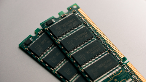
On the other hand, the RAM is in charge of storing the data that the CPU is about to consume. Of course the size of the RAM matters, but the speed of data transfer between the RAM and the CPU is also crucial. Nowadays, the typical size of the RAM ranges from 1 gigabyte to a few hundreds gigabytes.

For FEA, the RAM is important because it carries the model data: the stiffness matrix, the displacement vector and so on. The more degrees of freedom in the model, the more RAM is needed.

However, the number of time steps does not have a significant influence on the RAM consumed. As we will see in the next part, the time steps are solved sequentially, there is no need to store all of them on the RAM at the same time.

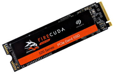
Finally, the hard drive is in charge of storing the model data that needs to persist after the FEA software execution, for instance: the resulting stress or strain fields. But the hard drive may also be implicated during the finite element resolution, when the RAM does not have enough room to handle all the data.

Therefore for FEA, a hard drive must propose enough storage capacity but also interesting read and write speed. Currently, the most appropriate solution is to use SSD (solid state drive) that combines both factors.

To conclude, the efficiency of a FEA software relies on 2 main factors: the execution speed and the computer RAM capacity:

• The execution speed is important to get FEA results in decent delays. It is mostly driven by the CPU and then the hard drive.
• While the RAM capacity is important to handle large FEA model.

I have not mentioned the GPU (graphic processing unit) here. It is currently a niche subject in the FEA world, but it is gaining more and more interest.

The importance of parallelization to improve FEA execution speed

Parallelization has gain a renewed interest in the recent years since the democratization of the multi-core CPU. The multi-core CPU possesses multiple computing units (called cores), each of them can process calculations at the same time. We then say that the calculations are parallelized. To benefit from parallel execution, a software must be able to distribute the calculations among the multiple CPU cores. And in order for the parallelization to be successful, each distributed calculation must be independent from the others.

Hopefully, there are multiple algorithms inside a FEA software that can be parallelized successfully. This comes from the very essence of the finite element method. For instance, to compute the stiffness matrix for a whole model, the first step is to compute the stiffness matrix for each element, and then assemble the results. And it turns out that each element’s stiffness matrix is independent from the others.

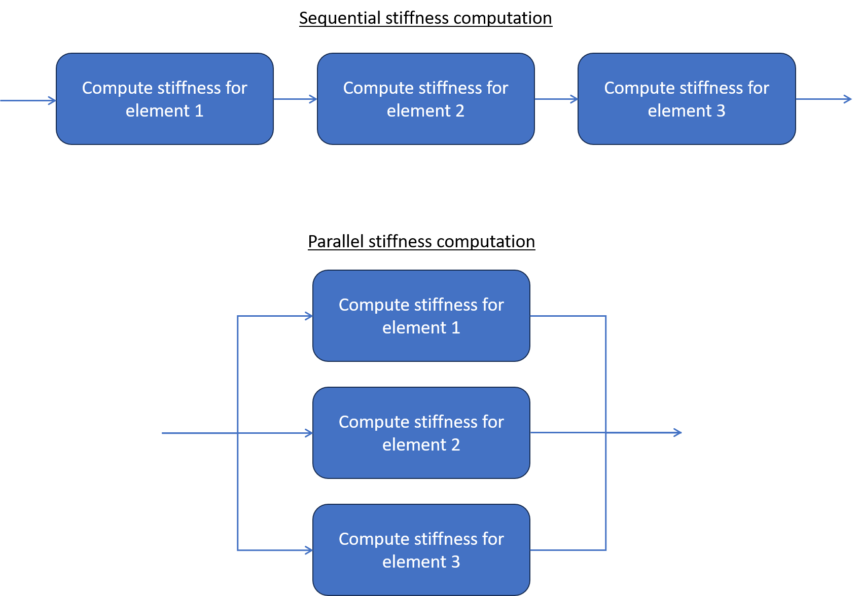
Basically, everything that is computed at the element level can benefit to some extent from parallelization. This means that in theory, parallelization can contain the increasing size of the model. In practice, there are always bottlenecks that prevent to fully achieve this objective, but a still interesting speed gain can be obtained.

On the other hand, FEA software cannot parallelize time steps resolution. Indeed, each time step depends on the previous one. They must be computed one after the other.

As we have seen previously, there are 2 factors that drives the number of computations required to perform a FEA resolution: the number of degrees of freedom and the number of time steps. Hence, a FEA resolution falls into one of the 4 possible scenarios:

• a small number of degrees of freedom and a small number of time steps –> Parallelization is useless but not really necessary because the execution time is small.
• a small number of degrees of freedom and a large number of time steps –> Parallelization is useless.
• a large number of degrees of freedom and a small number of time steps –> Parallelization is welcome because it is effective on large models.
• a large number of degrees of freedom and a large number of time steps –> Again, parallelization is welcome because it is effective on large models.

There exist other advanced techniques to benefit even more from parallelization. We can mention for instance the sub-domain decomposition technique, where the problem is decomposed into multiple sub-problems solved in parallel. Even though I have only touched on how FEA software can take advantage of parallelization, I hope I provided you the minimum knowledge to understand what is going inside FEA software. Whatever the parallelization technique, it is effective only on large models.

The differences between a workstation and a HPC cluster

Understanding the difference between a workstation and a HPC cluster is the first step to choose the right hardware for performing FEA.

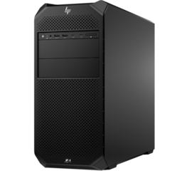
A workstation is very like a personal computer. Then main difference is that the workstation is composed of high-end components that are designed to handle high workloads without failing.

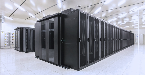
A HPC cluster can be seen as multiple workstations linked on a high speed network. In the HPC terminology, each workstation is called a node.

The following table compares a typical HPC cluster node resources with a typical workstation resources.

Of course you can find workstations or cluster nodes that are not in this table. But it still gives the general picture. In general a cluster node has more CPU cores and RAM available than a workstation.

Hence, a cluster node is able to handle larger models compared to a workstation:

• it has more RAM to handle higher number of degrees of freedom.
• it has more CPU cores to better parallelize the execution.

However, the true difference between a workstation and a HPC cluster is that the HPC cluster is able to make its nodes, themselves, work in parallel (if the software is designed for of course). Which increases even more the cluster capacity, in terms of number of degrees of freedom it can carry, and in terms of parallelization it can achieve.

If there is one thing to remember: HPC clusters are war machines that can handle efficiently very large models. But as long as your workstation capacity is not exceeded, there is no clear need to upgrade to a HPC cluster.

Choosing the right hardware to perform FEA

Let’s now get to the main topic. Choosing the right hardware to perform FEA is an incremental procedure. The best way to start is to simply use the computer that you already own. Be it, a laptop, a PC or a workstation, it can already provide useful information for the FEA jobs you are trying to solve:

• is it executing in a descent amount of time? If no, you will be looking for a more powerful CPU.
• is it overflowing the RAM capacity? If yes, you will be looking for more RAM.

From my experience, with a laptop or PC composed of:

• 2 GHz - 3 GHz CPU with 2 to 4 cores,
• 8 GiB of RAM,
• Hard drive (no SSD). You can handle FEA models up to a 1 million degrees of freedom.

If you already have a configuration close to the previous one, and you want to handle larger models, the best bet is simply to upgrade it:

• upgrade the RAM (with 32 GiB you can handle up to 5 million degrees of freedom),
• keep your hard drive but add a SSD.

It is important that you install the operating system and the useful software onto the SSD. Besides, when running FEA, make sure that the FEA data is also on the SSD. You do not need a very large SSD, usually 250 GiB to 500 GiB is enough. You can couple the SSD with a large hard drive (2 TiB for instance), so that you have enough space to store FEA results once they are computed.

If your current configuration is way below what I mentioned above, you can consider buying a new one. My advice is to look directly for a workstation instead of a PC. The following configuration is fine for models up to 5 million degrees of freedom, hence it allows to comfortably start doing FEA:

• 3 GHz CPU with 6 cores or more,
• 32 GiB of RAM,
• SSD + hard drive.

If possible, try to buy a workstation with empty slots available to add more RAM. So that you will be able to upgrade it, without needing to buy a whole new workstation.

Of course, if you seek to buy a brand new workstation it can cost a lot: the configuration mentioned previously sits somewhere between 1500€ and 3000€. My advice is to look for a refurbished workstation (on websites like backmarket or ebay for instance). These workstations mostly come from enterprises that renew their IT equipment. The previous configuration, in good shape, will cost from 500€ to 1000€.

If you need to tackle larger model, then try to find a workstation with more RAM (64 GiB or even 128 GiB). If you need even more RAM, then it is probably time for you to consider a HPC cluster solution.

Illustration of FEA performance on a workstation using the SesamX software

Let’s now illustrate this article with the performance that a workstation can reach. Here we use SesamX to study the following I beam model. This beam is clamped at one end and subjected to a transverse load at the other end.

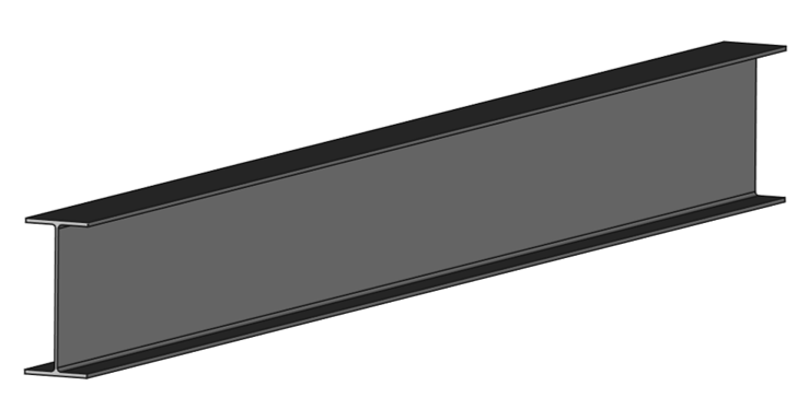
The beam is meshed using quadratic tetrahedron elements using multiple element sizes (from coarse to fine meshes). A simple linear static analysis is performed (i.e. there is only one time-step). The aim is to analyze the influence of the model size (number of degrees of freedom) on the execution time and the RAM consumed.

This analysis is performed on a HP Z320 workstation (running on Windows 10) composed of:

• 3.2 GHz CPU with 4 cores (Intel Xeon E3-1225 v3),
• 32 GiB of RAM,
• SSD

Five model sizes are analyzed:

• 110 Kdof,
• 1.3 Mdof,
• 2.5 Mdof,
• 3.5 Mdof,
• 4.7 Mdof.

First, the analysis is performed using 1 core only. The following figure gives the RAM consumed versus the number of degrees of freedom.

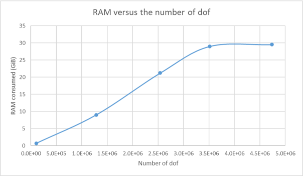
It is interesting to note that the RAM consumed depends linearly on the number of degrees of freedom. We can observe an inflection on the curve for the 4.7 Mdof model. As SesamX ran without memory error, I did not investigate any further. 30 GiB is the maximum RAM that can be used by SesamX (because around 2 GiB is constantly used by the operating system). My guess is that the 4.7 Mdof model is using swap memory that is not accounted for on the RAM value.

Afterwards, the analysis is performed using 2, 3 and 4 cores. First thing to note, the number of cores does not influence the RAM consumed. The following figure gives the execution time versus the number of degrees of freedom, for the 1, 2, 3 and 4 cores cases.

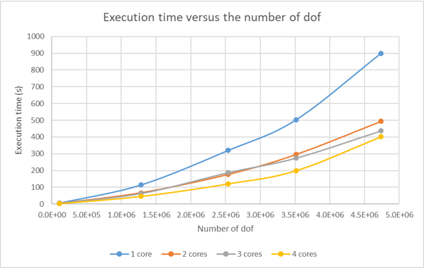
As we can see, the execution time depends quadratically on the number of degrees of freedom (regardless of the number of cores). And as the number of cores increases, the execution time decreases. Besides, we see that the performance gain is almost optimal when using 2 cores: the execution time decreases by 45% (where the optimal gain would be 50%) on the 4.7 Mdof model. Adding more cores has a benefit effect but in a smaller proportion. This last figure, depicting the execution time versus the number of cores (for the 4.7 Mdof model), illustrates clearly the previous statement.

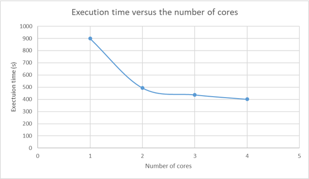
To conclude, this performance analysis showcases the important trends when parallelizing a FEA resolution:

• the RAM consumed does not depend on the number of cores.
• at one point, adding more cores does not decreases substantially the execution time. Finally, to echo the previous part about choosing the right hardware for FEA, the workstation used for this analysis is clearly limited in term of RAM. Without more RAM, there is no way to handle a model larger than 5 Mdof. Whereas the execution time remains decent thanks to parallelization.

To reproduce this simulation on your own, you can find:

• the I-beam step file
• the SesamX input files
• and the 110 Kdof model mesh

Conclusion

I hope this article provides you relevant information about why hardware is important for FEA, and on which hardware components you should focus. As I tried to demonstrate, the current hype around HPC cluster should not push us to forget about what we can achieve with a simple workstation, for far less money.