Facing the finite element method for the first time can be a bit frustrating. Indeed, there are multiple mathematical topics to master before understanding what is going on under the hood. Nevertheless, this is also the reason why the finite element method is so powerful: it builds a reliable bridge between abstract equations and concrete engineering applications.
This article aims at introducing the finite element method from a mathematical point of view. We are about to dive into algebra, tensor calculus and calculus of variations. We will take the linear elasticity problem as the support problem for this article. In the end you will get the whole picture about the finite element method and how you can start implementing it in a computer software. And if you seek to go further about the finite element method, I share 2 good references to read at the end of this article.
If you are looking for a more general introduction about the finite element method, I advise you to watch the best video I ever found on this subject.
You can also consult the following articles to get a more practical presentation about specific finite elements:
Quick remark on notations
Before starting, let’s define some notations that are used through this article:
vectors are denoted with an underline $ \underline{u} $ , second order tensors with a double underline $ \underline{\underline{\varepsilon}} $ and so on,
matrices are represented with brackets,
unless otherwise indicated, Einstein summation convention is used on repeated indices,
partial derivatives are denoted with the comma notation $ u_{,x} $ .
The finite element method applied to the elasticity problem
Before diving into the finite element method, let’s give some background information about the elasticity problem. Our ultimate goal is to solve the following partial differential equation (PDE) for the displacement $ \underline{u} $ on a solid occupying the domain $ \Omega $ :
$$ \begin{alignedat}{2} \underline{\nabla} \cdot \underline{\underline{\sigma}}(\underline{u}) = 0 &, \ \ \ & \underline{x} \in \Omega \\ \underline{u} = 0 &, \ \ \ & \underline{x} \in \Gamma_h \\ \underline{\underline{\sigma}} \cdot \underline{n} = \underline{t} &, \ \ \ & \underline{x} \in \Gamma_s \end{alignedat} $$
Where:
$ \underline{x} $ denotes the position vector,
$ \underline{\underline{\sigma}} $ denotes the stress tensor,
$ \Gamma_h $ is the part of the frontier on which the displacement is prescribed to 0,
$ \Gamma_s $ is the part of the frontier on which the surface traction $ \underline{t} $ is applied,
and $ \underline{n} $ denotes the outward normal of the domain frontier.
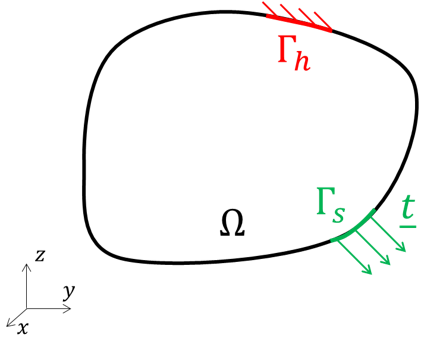
This equation is called the strong form of the elasticity problem.
We also introduce the infinitesimal strain tensor, defined as:
$$ \underline{\underline{\varepsilon}} = \cfrac{1}{2} (\underline{\underline{\nabla u}} + \underline{\underline{\nabla u}}^T) $$
And the material law (Hooke’s law) between the stress and the strain tensors:
$$ \underline{\underline{\sigma}} = \underline{\underline{\underline{\underline{C}}}} : \underline{\underline{\varepsilon}}, \ \ \ \text{with} \ \ \ \underline{\underline{\underline{\underline{C}}}} = \lambda \underline{\underline{I}} \otimes \underline{\underline{I}} + 2 \mu \underline{\underline{I}} $$
Where:
- $ \lambda $ and $ \mu $ are the Lamé constants,
- and $ \underline{\underline{I}} $ is the second-order identity tensor.
In order to solve this problem we need:
a mathematical description of the solid domain,
and a mathematical resolution procedure to solve the partial differential equation on this domain.
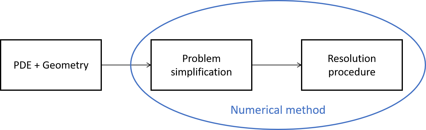
Unfortunately, closed-form solutions usually do not exist for complex domain. One way to circumvent this issue is to simplify the problem, and then solve in closed-form this simplified problem. Off course, we want the simplified problem to be as close as possible to the initial problem, which would ensure that the solution obtained is a reliable approximate solution to the initial problem.
In other words, the main philosophy adopted is to trade problem simplification with approximation in the solution, while keeping the problem close to the original one.
Hence we define a numerical method as a tool that proposes simplifications of a mathematical problem, as well as the associated solving procedure.
Over time, multiple numerical methods have been proposed to solve the elasticity problem. The major ones are: the finite difference method, the finite volume method and the finite element method. Mainly because of mathematical and practical reasons, the finite element method has proven to be the best suited to solve efficiently elasticity problems.
The finite element method brings 2 main simplifications to the original problem: one on the domain discretization, and the other on the equation solved. These simplifications are detailed in the following.
Domain discretization with finite elements
Real world solid domain can be of infinite complexity. And the first step is to derive a mathematical description of this domain. Which is done with a mesh discretizing the domain.
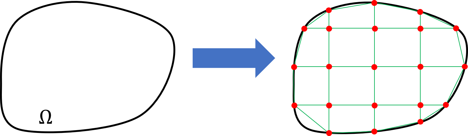
The mesh is made of nodes (the red points) linked together to form elements (the green cells). As you can see, the mesh is an idealization of the underlying domain. While controlling the mesh fineness, we can get a closer mathematical description of the domain.
Usually, the mesh is built by a computer program called a mesher. The goal of this program is to minimize both the deviation from the underlying domain and the number of nodes. However, this process cannot be 100% automatic and requires user interaction. Indeed it is the user responsibility to decide which details need to be kept and which need to be left. Furthermore, the problem resolution depends on the mesh: the finer the mesh, the more computing resources are required to solve the problem. To summarize, building a mesh means finding a compromise between representativeness and performance.
Depending on the problem considered, a mesh is composed of 1D, 2D or 3D elements.

This article focuses on the 3D elasticity problem. However, for sake of simplicity the illustrations will often showcase 2D elements. The idea gained from these illustrations can of course be extrapolated to 3D or 1D elements.
Once the mesh is built, the next step is to solve the problem equation.
Derivation of the problem’s weak form
In this part, we are going to restate the problem and derive a new expression of the governing equation, equivalent to the strong form. This new expression is called the weak form (as opposed to the strong form) for reasons that we will discuss in the following. Obtaining the weak form is the starting point of the finite element method, on which further simplifications are applied.
There are multiple equivalent approaches to obtain the weak form. For this article I chose the approach that I find the most physical. This approach is often called the energy approach.
Problem statement
First, let’s restate the problem. We seek to compute the displacement vector $ \underline{u}(x, y, z) $ at every location inside the solid. Under the prescribed displacement on $ \Gamma_h $ and the prescribed surface traction on $ \Gamma_s $ .
From now on, we will not consider the partial differential equation provided above. We will look at the problem from an energy point of view and apply Hamilton’s principle.
Applying Hamilton’s principle
To apply Hamilton’s principle, we need first the energy balance of the system.
Energy balance
On one hand there is the energy stored in the solid as a result of the deformation:
$$ V(\underline{u})=\int_\Omega \cfrac{1}{2} \ \underline{\underline{\varepsilon}} : \underline{\underline{\sigma}} \ d\Omega $$
And on the other hand, there is the work done by the external forces:
$$ W(\underline{u}) = \int_{\Gamma_s} \underline{t} \cdot \underline{u} \ d\Gamma $$
We can therefore write the energy balance $ E(\underline{u}) $ of the system as:
$$ E(\underline{u}) = V(\underline{u}) - W(\underline{u}) = \int_\Omega \cfrac{1}{2} \ \underline{\underline{\varepsilon}}(\underline{u}) : \underline{\underline{\sigma}}(\underline{u}) \ d\Omega - \int_{\Gamma_s} \underline{t} \cdot \underline{u} \ d\Gamma $$
Eventually, inserting the Hooke’s law yields the following expression for the energy balance:
$$ \boxed{ E(\underline{u}) = \int_\Omega \cfrac{1}{2} \ \underline{\underline{\varepsilon}}(\underline{u}) : \underline{\underline{\underline{\underline{C}}}} : \underline{\underline{\varepsilon}}(\underline{u}) \ d\Omega - \int_{\Gamma_s} \underline{t} \cdot \underline{u} \ d\Gamma } $$
It is clearly apparent that this energy balance depends only on the displacement.
$ E(\underline{u}) $ is a functional. It takes on input a function (the displacement $ \underline{u} $ ) and gives on output a scalar (the energy balance). Some people may also use the term “function of function”. In the following, we are going to manipulate the $ E(\underline{u}) $ functional in order to find its minimum.
Hamilton principle
Once we have the energy balance, we can apply Hamilton’s principle.
This principle states that: if we find a displacement $ \underline{u} $ that minimizes the energy balance $ E(\underline{u}) $ , then this displacement is a solution to the problem.
To find the minimum of the functional $ E(\underline{u}) $ , we need to introduce the notion of functional variation.
For an arbitrary function $ \delta \underline{u} : \Reals^3 \to \Reals^3 $ which is differentiable, the variation of $ E $ at $ \underline{u} $ in the direction $ \delta \underline{u} $ is defined by:
$$ \delta E(\underline{u}, \delta \underline{u}) = \lim\limits_{t \to 0} \cfrac {E(\underline{u} + t \delta \underline{u}) - E(\underline{u})} {t} $$
$ \delta E(\underline{u}, \delta \underline{u}) $ can be seen as the directional derivative of $ E $ at $ \underline{u} $ in the direction $ \delta \underline{u} $ .
If we go back to the minimization problem, it can be shown that finding the displacement $ \underline{u} $ that minimizes $ E(\underline{u}) $ is equivalent to finding the displacement $ \underline{u} $ that solves the following equation:
$$ \delta E(\underline{u}, \delta \underline{u}) = 0, \ \ \ \forall \delta \underline{u} $$
The clause $ \forall \delta \underline{u} $ is tremendously important here. We can restate this equation as: if the directional derivative of $ E $ at $ \underline{u} $ is $ 0 $ in every possible direction $ \delta \underline{u} $ , then $ \underline{u} $ is the solution.
Hence using the symmetry of $ \underline{\underline{\underline{\underline{C}}}} $ and $ \underline{\underline{\varepsilon}} $ , Hamilton’s principle translates to:
$$ \boxed{ \int_\Omega \underline{\underline{\varepsilon}}(\underline{u}) : \underline{\underline{\underline{\underline{C}}}} : \delta(\underline{\underline{\varepsilon}}(\underline{u})) \ d\Omega = \int_{\Gamma_s} \underline{t} \cdot \delta \underline{u} \ d\Gamma , \ \ \ \forall \delta \underline{u} } $$
This form of the elasticity problem is called the weak form.
As can be seen, the strong form states the elasticity problem at each point of the domain. Whereas the weak form states the problem in an average sense through the integral. It can be shown that both forms are equivalent. Hence, no simplification are made during the weak form derivation.
As mentioned previously, the finite element method seeks to simplify the original problem in order to solve it. It applies simplifications on the weak form in order to degrade the problem globally. Whereas applying simplifications on the strong form would degrade the problem locally. This is one of the reasons why the finite element method is so efficient.
Expression of the weak form in tensor components
To make things easier we will work with vector and tensor components in the global basis $ (\underline{e_1}, \underline{e_2}, \underline{e_3}) $ (associated with the coordinate system $ (x,y,z) $ ) instead of the tensor and vector notations.
For a vector, such as the displacement vector we have:
$$ \underline{u} = u_i \underline{e_i} $$
For a second order tensor, such as the strain tensor we have:
$$ \underline{\underline{\varepsilon}} = \varepsilon_{ij} \underline{e_i} \otimes \underline{e_j} $$
For a fourth order tensor, such as the material tensor we have:
$$ \underline{\underline{\underline{\underline{C}}}} = C_{ijkl} \underline{e_i} \otimes \underline{e_j} \otimes \underline{e_k} \otimes \underline{e_l} $$
From the definition of the infinitesimal strain tensor, we can write:
$$ \varepsilon_{ij} = \cfrac{1}{2} (u_{i,j} + u_{j,i}) $$
And similarly:
$$ \delta \varepsilon_{kl} = \cfrac{1}{2} (\delta u_{k,l} + \delta u_{l,k}) $$
Inserting all this into the weak form we get:
$$ \int_\Omega \cfrac{1}{2} (u_{i,j} + u_{j,i}) \ C_{ijkl} \ \cfrac{1}{2} (\delta u_{k,l} + \delta u_{l,k}) \ d\Omega = \int_{\Gamma_s} t_i \delta u_i \ d\Gamma, \ \ \ \forall (\delta u_1, \delta u_2, \delta u_3) $$
All the indices in the previous expression are dummy indices, we can then rearrange the terms and factorize the expression.
$$ \int_\Omega \cfrac{1}{4} u_{i,j} (C_{ijkl} + C_{jikl} + C_{ijlk} + C_{jilk}) \delta u_{k,l} \ d\Omega = \int_{\Gamma_s} t_i \delta u_i \ d\Gamma, \ \ \ \forall (\delta u_1, \delta u_2, \delta u_3) $$
And using the symmetry of the material tensor:
$$ C_{ijkl} = C_{jikl} = C_{ijlk}, \ \ \ \forall (i, j, k, l = 1, 2, 3) $$
We finally obtain the weak form in components notation:
$$ \boxed{ \underbrace{\int_\Omega u_{i,j} C_{ijkl} \delta u_{k,l} \ d\Omega }_{\text{internal work integral}} = \underbrace{\int_{\Gamma_s} t_i \delta u_i \ d\Gamma }_{\text{external work integral}}, \ \ \ \forall (\delta u_1, \delta u_2, \delta u_3) } $$
Where, for practical reasons, we have identified the internal work part and the external work part.
Simplification of the weak form
As for the strong form, we cannot derive a closed-form solution from the weak form. The next step of the finite element method is to simplify the weak form as explained below.
Displacement interpolation inside each element
The major difficulty is to find a displacement function satisfying both the weak form and the prescribed condition on the domain frontier. One, solution is to assume a specific interpolation for the displacement inside each element of the mesh, instead of looking for the exact displacement function.
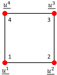
$$ \underline{u(x, y, z)} = N^I(x, y, z) \underline{u^I} $$
Where:
- $ \underline{u^I} $ is the displacement vector at the element’s $ I^{th} $ node,
- and $ N^I $ is the interpolation function associated with the element’s $ I^{th} $ node.
We defer to the end of this article the details about how the $ N^I $ functions are obtained.
In components notation this interpolation translates to (the dependence on $ x, y, z $ is considered implicit):
$$ u_i = N^I u_i^I $$
As we can see, the parameters driving this interpolation are the displacements at the nodes. Therefore, once we know the displacements at the nodes, we can express the displacement at any point inside the element. And to stay consistent, we use the same interpolation for $ \delta \underline{u} $ and $ \underline{u} $ .
Factorization of the weak form inside each element
From the specific displacement interpolation inside each element, it is interesting to split the weak form integral into a sum of integrals over each element domain. It will then be easier to rework each element’s integral independently, before assembling the results (as explained in the next section).
$$ \int_\Omega \dots \ d\Omega = \int_{\Gamma_s} \dots d\Gamma $$
$$ \iff $$
$$ \sum_{1 \leq e \leq N_e} \int_{\Omega_e} \dots \ d\Omega = \int_{\Gamma_{s_e}} \dots d\Gamma $$
Where:
- $ \Omega_e $ is the domain of the $ e^{th} $ element,
- $ \Gamma_{s_e} $ is the frontier of the $ e^{th} $ element domain on which a surface traction is applied,
- and furthermore, from now on we consider that the mesh is made of $ N_n $ nodes and $ N_e $ elements.
We may drop some $ e $ indices in the following of this section to avoid unnecessary complication. For the remaining of this section, it is implied that we are working at the element level. The number of nodes of the element will be denoted with $ N_{n_{elem}} $ .
Element internal work integral
Once we insert the displacement interpolation into the element internal work integral we get:
$$ \int_{\Omega_e} u_i^I N_{,j}^I C_{ijkl} N_{,l}^J \delta u_k^J \ d\Omega $$
This integral showcases a bilinear relation between $ u_i^I $ and $ \delta u_k^J $ (considering $ I $ and $ J $ fixed). For every couple of nodes $ (I, J) $ (no summation on $ I $ and $ J $ in the following expression), we can write:
$$ \int_{\Omega_e} u_i^I N_{,j}^I C_{ijkl} N_{,l}^J \delta u_k^J \ d\Omega = \underbrace{ \begin{bmatrix} \delta u_1^J \\\\ \delta u_2^J \\\\ \delta u_3^J \end{bmatrix}^T }_{[\delta U^{J}]^T} \underbrace{ \begin{bmatrix} K_{11}^{JI} & K_{12}^{JI} & K_{13}^{JI} \\\\ K_{21}^{JI} & K_{22}^{JI} & K_{23}^{JI} \\\\ K_{31}^{JI} & K_{32}^{JI} & K_{33}^{JI} \end{bmatrix} }_{[K^{JI}]} \underbrace{ \begin{bmatrix} u_1^I \\\\ u_2^I \\\\ u_3^I \end{bmatrix} }_{[U^{I}]} $$
With
$$ K_{ki}^{JI} = \int_{\Omega_e} N_{,j}^I C_{ijkl} N_{,l}^J \ d\Omega $$
If we stack all the element nodal displacements in the same column matrix we can write:
$ [\delta U_e] = \begin{bmatrix} [\delta U^1] \\\\ [\delta U^2] \\\\ \vdots \\\\ [\delta U^{N_{n_{elem}}}] \end{bmatrix}, \ \ \ [U_e] = \begin{bmatrix} [U^1] \\\\ [U^2] \\\\ \vdots \\\\ [U^{N_{n_{elem}}}] \end{bmatrix} $And $ [K_e] = \begin{bmatrix} [K^{11}] & [K^{12}] & [K^{13}] & \dots & [K^{1{N_{n_{elem}}}}] \\\\ [K^{21}] & [K^{22}] & [K^{23}] & \dots & [K^{2{N_{n_{elem}}}}] \\\\ \vdots & \vdots & \vdots & \vdots & \vdots \\\\ [K^{{N_{n_{elem}}}1}] & [K^{{N_{n_{elem}}}2}] & [K^{{N_{n_{elem}}}}] & \dots & [K^{{N_{n_{elem}}}{N_{n_{elem}}}}] \end{bmatrix} $
Therefore, the element internal work integral can be written as (this time with full summation on $i, j, k, l, I, J$ ):
$$ \boxed{ \int_{\Omega_e} u_i^I N_{,j}^I C_{ijkl} N_{,l}^J \delta u_k^J \ d\Omega = [\delta U_e]^T \ [K_e] \ [U_e] } $$
$ [K_e] $ is called the element stiffness matrix from the analogy with a spring force-displacement relation: $ f_{spring} = k_{spring} u_{spring} $ .
It should be noted that the element stiffness matrix is symmetric: $ [K_e] = [K_e]^T $ .
Element external work integral
Similarly, the element external work integral is given by:
$$ \int_{\Gamma_{s_e}} t_i N^I \delta u_i^I \ d\Gamma $$
This integral showcases a linear relation among $ u_i^I $ (considering $ I $ fixed). Hence, for every node $ I $ (no summation on $ I $ in the following expression), we can write:
$$ \int_{\Gamma_{s_e}} t_i N^I \delta u_i^I \ d\Gamma = \underbrace{ \begin{bmatrix} \delta u_1^J \\\\ \delta u_2^J \\\\ \delta u_3^J \end{bmatrix}^T }_{[\delta U^{I}]^T} \underbrace{ \begin{bmatrix} F_1^I \\\\ F_2^I \\\\ F_3^I \end{bmatrix} }_{[F^{I}]} $$
With:
$$ F_i^I = \int_{\Gamma_{s_e}} t_i N^I \ d\Gamma $$
Similarly to the internal work integral, if we stack all the element nodal forces in the same column vector, we have:
$$ [F_e] = \begin{bmatrix} [F^1] \\\\ [F^2] \\\\ \vdots \\\\ [F^N] \end{bmatrix} $$
Therefore, the element external work integral can be written as (this time with full summation on $i, I$ ):
$$ \boxed{ \int_{\Gamma_{s_e}} t_i N^I \delta u_i^I \ d\Gamma = [\delta U_e]^T \ [F_e] } $$
$ [F_e] $ is called the element force column matrix.
Assembly of each element contribution
Summing up the stiffness and force contribution from each element, we can express the weak form as follows:
$$ \sum_{1 \leq e \leq N_e} [\delta U_e]^T \ [K_e] \ [U_e] = \sum_{1 \leq e \leq N_e} [\delta U_e]^T \ [F_e], \ \ \ \forall [\delta U_e], 1 \leq e \leq N_e $$
Each element contribution to the weak form was derived independently from the other elements. Nevertheless, the elements are not independent from each other. Indeed, neighbors elements share some of their nodes. Therefore we can factorize further the previous relation while summing the element contributions at the nodes. This process is called the assembly.
Once the assembly is performed, the weak form becomes:
$$ [\delta U]^T \ [K] \ [U] = [\delta U]^T \ [F], \ \ \ \forall [\delta U] $$
Where:
- $ [U] $ represents the column matrix for the displacements at each node of the mesh (similarly for $ [\delta U] $ ).
$$ [U] = \begin{bmatrix} [u^1] \\\\ [u^2] \\\\ \vdots \\\\ [u^{N_n}] \end{bmatrix}, \ \ \ \text{with} [u^i] = \begin{bmatrix} u_1^i \\\\ u_2^i \\\\ u_3^i \end{bmatrix} $$
- $ [F] $ represents the column matrix for the force at each node of the mesh.
$$ [F] = \begin{bmatrix} [f^1] \\\\ [f^2] \\\\ \vdots \\\\ [f^{N_n}] \end{bmatrix}, \ \ \ \text{with} [f^i] = \begin{bmatrix} f_1^i \\\\ f_2^i \\\\ f_3^i \end{bmatrix} $$
- and $ [K] $ represents the global stiffness matrix (its size is $ N_n \times N_n $ )
Because the weak form must hold for all $ [\delta U] $ , it is equivalent to require:
$$ \boxed{ [K] \ [U] = [F] } $$
Inverting the previous relation, we get the displacement at each node of the model. Furthermore, using the element displacement interpolation we are able to provide the displacement at each point of the solid. Which terminates the finite element procedure.
However, there are still 2 shadow areas that we have not yet explained:
- obviously we need to know the $ N^I $ interpolation functions. How do we get them?
- how can we evaluate the integrals relying on arbitrary element domains?
These 2 topics are addressed conjointly in the following section.
Finite element integrals evaluation
In order to effectively apply the finite element method, we need to evaluate the stiffness matrix and force column matrix for each element. It appears that the components of the element stiffness matrix are made of integrals over the element domain (and similarly for the element force column matrix). However, in the general case, these integrals cannot be computed analytically. Therefore we need specific methods that are both precise and computationally efficient to evaluate these integrals.
To illustrate our explanation, we will consider the following distorted 2D element.

As the integral computation procedures are similar between the stiffness matrix terms and the force matrix terms, we only focus on the stiffness matrix terms computation here. The typical integral to compute is therefore:
$$ \boxed{ K_{ki}^{LK} = \int_{\Omega_e} g^{LK}(x,y) \ d\Omega } $$
With:
$$ g^{LK}(x,y) = N_{,j}^K(x,y) C_{ijkl} N_{,l}^L(x,y) $$
To evaluate the integral over the element domain, we need to apply a quadrature rule. The goal of a quadrature rule is to evaluate the integral while probing the integrand at specifically chosen locations.
Considering the following function $ f: x,y \to f(x,y) $ , a quadrature rule states that:
$$ \int_{x=-1}^{1}\int_{y=-1}^{1} f(x,y) \ dxdy \approx \sum_{i=1}^n w_i f(x_i, y_i) $$
Where:
- the couples $ (x_i, y_i) $ are the probing points of the quadrature rule,
- the $ w_i $ are the weights associated to each probing point,
- $ n $ is the number of probing points.
To put it simply, the more probing points, the better the accuracy. Besides, multiple quadrature rules exist, each having its advantages and disadvantages. Usually, Gaussian quadrature is used.
As we can see in the previous formula, the quadrature rule is provided for a rectangular integral domain. Which is not the case of the distorted element shape. However, this is not an issue. We can find a suitable change of variables that will transform the integral as desired. This change of variables is also called a mapping, because it maps the element in the $ (x,y) $ coordinates with the same element described in $ (r,s) $ coordinates. If we rectangularize the $ (r,s) $ coordinates representation, the mapping can be illustrated as follows:
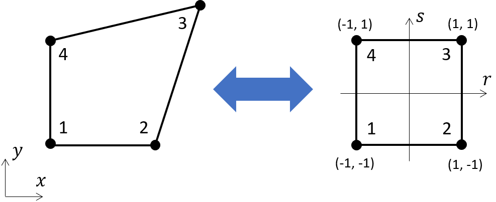
There can be an infinity of valid mappings. However, in the case of the 4-node quad element, the most prevalent approach is to adopt a bilinear mapping (in $ r $ and $ s $ ).
To define this mapping we rely on shape functions defined in the $ (r,s) $ coordinates. Each shape function is associated to a node on the element. Furthermore, for each shape function $ \widetilde{N^I}(r,s) $ (associated to the $ I^{th} $ node on the element) we require:
$$ \begin{cases} \widetilde{N^I}(r_J,s_J) = 0, \ \ \ \forall J = \not I \\ \widetilde{N^I}(r_I,s_I) = 1 \end{cases} $$
And the mapping to adopt must linearly depend on the element’s nodes position:
$$ \boxed{ \begin{cases} x(r,s) = \widetilde{N^I}(r,s) x_I \\ y(r,s) = \widetilde{N^I}(r,s) y_I \end{cases} } $$
For the 4-node quad element, in can be shown that there is only one bilinear mapping satisfying the requirements. Which is the following:
$$ \begin{cases} \widetilde{N^1}(r,s) = \cfrac{1}{4}(1-r)(1-s) \\ \widetilde{N^2}(r,s) = \cfrac{1}{4}(1+r)(1-s) \\ \widetilde{N^3}(r,s) = \cfrac{1}{4}(1+r)(1+s) \\ \widetilde{N^4}(r,s) = \cfrac{1}{4}(1-r)(1+s) \end{cases} $$
Finally, we can rewrite the stiffness integrals using the mapping previously defined as:
$$ \int_{\Omega_e} g^{LK}(x,y) d\Omega = \int_{-1}^1\int_{-1}^1 \widetilde{g^{LK}}(r,s) |det(J(r,s))| drds $$
Where:
- $ \widetilde{g^{LK}}(r,s) = g^{LK}(x(r,s), y(r,s)) $
- and $ det(J(r,s)) $ is the determinant of the Jacobian matrix defined as
$$ [J(r,s)] = \begin{bmatrix} \cfrac {\partial x}{\partial r} & \cfrac {\partial x}{\partial s} \\\\ \cfrac {\partial y}{\partial r} & \cfrac {\partial y}{\partial s} \end{bmatrix} = \begin{bmatrix} \cfrac {\partial \widetilde{N^I}}{\partial r} x_I & \cfrac {\partial \widetilde{N^I}}{\partial s} x_I \\\\ \cfrac {\partial \widetilde{N^I}}{\partial r} y_I & \cfrac {\partial \widetilde{N^I}}{\partial s} y_I \end{bmatrix} $$
Eventually, the quadrature formula is given by:
$$ \boxed{ \int_{\Omega_e} g^{LK}(x,y) d\Omega = \sum_{i=1}^n w_i \widetilde{g^{LK}}(r_i,s_i) |det([J(r_i,s_i)])| } $$
Isoparametric finite element
To actually compute the integral provided above, we need the expression for $ \widetilde{g^{LK}}(r_i,s_i) $ . From the definition of $ \widetilde{g^{LK}} $ , we have:
$$ \widetilde{g^{LK}}(r,s) = N_{,j}^K(x,y) \ C_{ijkl} \ N_{,l}^L(x,y) $$
Where it is implied that $ x $ and $ y $ depend on $ r $ and $ s $ (using the mapping previously defined), and the $ N^K $ functions are the interpolation functions for the displacement in the $ (x,y) $ coordinates.
When first mentioning the $ N^K $ functions, we skillfully avoided to provide their explicit expression. Indeed they were not essential to the derivation that followed. However, it is now time to provide more details.
As for the mapping that we built between the $ (x,y) $ coordinates and the $ (r,s) $ coordinates, we have an infinite number of choices for the functions $ N^K $ . The key idea behind the iso-parametric element, is to use the same shape function for the displacement interpolation as for the coordinate mapping. In other words we choose:
$$ N^K(x,y) = \widetilde{N^K}(r,s) $$
The displacement is then interpolated using the shape functions expressed in the $ (r,s) $ coordinates. Even though we cannot give an explicit formula for $ N^K(x,y) $ , we know that this function exists because of the mapping between the $ (x,y) $ coordinates and the $ (r,s) $ coordinates.
Hence, we can rewrite the stiffness terms as:
$$ \boxed{ K_{ki}^{LK} = \sum_{i=1}^n w_i \widetilde{N_{,j}^K}(r_i,s_i) \ C_{ijkl} \ \widetilde{N_{,l}^L}(r_i,s_i) |det([J(r_i,s_i)])| } $$
The last difficulty is to compute the terms $ \widetilde{N_{,j}^K} = \cfrac{\partial \widetilde{N^K}} {\partial x_j}, \ \ \ \forall K,j $ .
However, using the chain-rule yields:
$$ \begin{cases} \cfrac{\partial \widetilde{N^K}} {\partial r} = \cfrac{\partial \widetilde{N^K}} {\partial x} \cfrac{\partial x} {\partial r} + \cfrac{\partial \widetilde{N^K}} {\partial y} \cfrac{\partial y} {\partial r} \\\\ \cfrac{\partial \widetilde{N^K}} {\partial s} = \cfrac{\partial \widetilde{N^K}} {\partial x} \cfrac{\partial x} {\partial s} + \cfrac{\partial \widetilde{N^K}} {\partial y} \cfrac{\partial y} {\partial s} \end{cases} $$
That we can rewrite as:
$$ \begin{bmatrix} \cfrac{\partial \widetilde{N^K}} {\partial r} \\\\ \cfrac{\partial \widetilde{N^K}} {\partial s} \end{bmatrix} = \begin{bmatrix} \cfrac{\partial x} {\partial r} & \cfrac{\partial y} {\partial r} \\\\ \cfrac{\partial x} {\partial s} & \cfrac{\partial y} {\partial s} \end{bmatrix} \begin{bmatrix} \cfrac{\partial \widetilde{N^K}} {\partial x} \\\\ \cfrac{\partial \widetilde{N^K}} {\partial y} \end{bmatrix} $$
Where we recognize the Jacobian matrix previously mentioned. Inverting this system we get:
$$ \begin{bmatrix} \cfrac{\partial \widetilde{N^K}} {\partial x} \\\\ \cfrac{\partial \widetilde{N^K}} {\partial y} \end{bmatrix} = [J]^{-T} \begin{bmatrix} \cfrac{\partial \widetilde{N^K}} {\partial r} \\\\ \cfrac{\partial \widetilde{N^K}} {\partial s} \end{bmatrix} $$
That we can eventually insert back in the stiffness terms above. These terms can now be fully computed. The finite element derivation is complete.
There are 2 main advantages of the iso-parametric hypothesis:
as you can notice, it reuses the Jacobian matrix already computed for the mapping. Which is a good point in terms of computation performance.
and it can be shown that as long as the element uses the iso-parametric hypothesis, it will converge to the exact solution as the mesh is refined (independently of the element shape: quadrangle, triangle, …).
Conclusion
I hope this article provided you with a gradual exposure to the finite element method. While following the derivation provided here, you should be able to implement iso-parametric elements in a computer software. Finally if you seek to dive deeper into the finite element method I advise you to check the following references:
Which are 2 very good books about the finite element method, explaining also how to implement it in a computer program.
Annex: Example of finite element stiffness assembly
To illustrate how the assembly process works, let’s consider the following mesh.
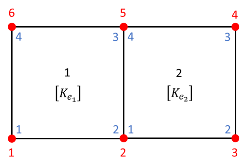
Where:
- global nodes number are denoted in red,
- element local nodes number are denoted in blue,
- element numbers are denoted in black,
- $ [K_{e_1}] $ is the stiffness matrix for the element 1 (and similarly for $ [K_{e_2}] $ ).
Detailing the full expression for $ [K_{e_1}] $ (in local nodes indices), we have:
$$ [K_{e_1}] = \begin{bmatrix} [K_{e_1}^{11}] & [K_{e_1}^{12}] & [K_{e_1}^{13}] & [K_{e_1}^{14}] \\\\ & [K_{e_1}^{22}] & [K_{e_1}^{23}] & [K_{e_1}^{24}] \\\\ sym & & [K_{e_1}^{33}] & [K_{e_1}^{34}] \\\\ & & & [K_{e_1}^{44}] \end{bmatrix} $$
An similarly for $ [K_{e_2}] $ .
From the mesh illustration, we note that the global nodes 1 and 6 are only connected through the element 1. Hence, the global stiffness terms on these 2 nodes will come only from element 1 (respectively for the global nodes 3 and 4 with the element 2).
However, the 2 elements share the global nodes 2 and 5. Hence the global stiffness terms on these 2 nodes will be the sum of each element contribution.
The resulting global stiffness matrix is therefore:
$$ [K] = \begin{bmatrix} [K_{e_1}^{11}] & [K_{e_1}^{12}] & 0 & 0 & [K_{e_1}^{13}] & [K_{e_1}^{14}] \\\\ & ([K_{e_1}^{22}]+[K_{e_2}^{11}]) & [K_{e_2}^{12}] & [K_{e_2}^{13}] & ([K_{e_1}^{23}]+[K_{e_2}^{14}]) & [K_{e_1}^{24}] \\\\ & & [K_{e_2}^{22}] & [K_{e_2}^{23}] & [K_{e_2}^{24}] & 0 \\\\ & & & [K_{e_2}^{33}] & [K_{e_2}^{34}] & 0 \\\\ & sym & & & ([K_{e_1}^{33}]+[K_{e_2}^{44}]) & [K_{e_1}^{34}] \\\\ & & & & & [K_{e_1}^{44}] \end{bmatrix} $$
Did you like this content?
Register to our newsletter and get notified of new articles