4. Post-processing

Once you have created an image file using SesamX, you can post-process its content. Similarly to the pre-processing, there can be multiple ways to post-process the content of an image file, and you are free to chose the workflow that works best for you. However, this page aims at exposing the preferred method to post-process SesamX images. It relies on the Salome software, and the SesamX viewer tool (a Salome add-in). Both of them enable efficient manipulations of the images content.

In order to have access to the SesamX viewer, you need to run the customized Salome version bundled in the SesamX installation archive. The information given below assumes that Salome is installed at the following location: “C:\SALOME-9.9.0” (for more details, please refer to the installation procedure).

First, you need to run Salome to access the SesamX viewer. To proceed, you have to double click on the “run_salome.bat” script or the “run_salome.exe” executable inside “C:\SALOME-9.6.0”. Afterward, you need to load the Paravis module as shown in the following picture.

Once loaded, you should see the following screen.

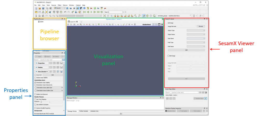
Only the relevant panels for post-processing SesamX images are highlighted in the previous picture:

• the SesamX viewer panel that enables visualization creation and modification.
• the pipeline browser that organizes the various visualizations created.
• the properties panel that contains options to control the visualizations.
• and the visualization panel that display the visualizations.

Only the SesamX viewer panel is part of the customization. The other components are embedded in the default Salome version.

The Paravis module of Salome relies on the Paraview software. Hence, Paravis shares multiple features with Paraview. The remaining of this page will mainly discuss the SesamX viewer panel, plus some Paraview tips. The goal is to teach you how to create visualizations efficiently from SesamX images files. If you are looking for more information about Paraview features and manipulation, we advise you to consult the Paraview website.

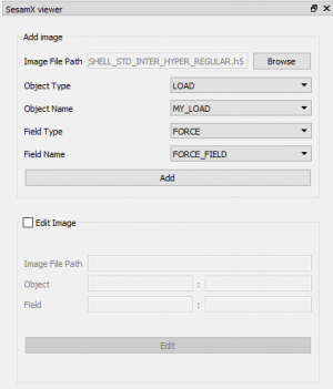
To create a visualization, the first step is to load an image file with the “Browse” button. The following combo boxes (“Object Type”, “Object Name”, “Field Type” and “Field Name”) let you chose which field you want to visualize from the image file. These combo boxes work in a cascading manner: once you have chosen the “Object Type”, it will update the available options for the “Object Name”, once you have chosen the “Object Name”, it will update the available options for the “Field Type” and so on. Hence they allow you to narrow down the field search:

• First, the “Object Type” lets you chose the type of the SesamX object holding the desired field (characteristic, constraint, load or solution).
• Then, the “Object Name” lets you chose the name of the SesamX object associated to the field you are looking for.
• Then, the “Field Type” lets you chose the type of field available on this object.
• And finally the “Field Name” lets you select the field you want to visualize.

For instance, to select the “FORCE” field named “FORCE_FIELD” from the “LOAD” object named “MY_LOAD”, we have to select:

Finally, you can click on the “Add” button to create the visualization. The visualization will appear in the visualization panel, as well as in the pipeline browser.

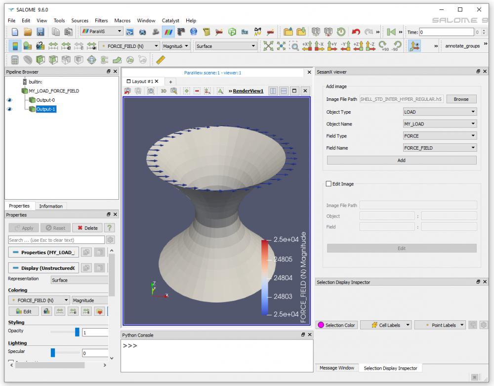
In the pipeline browser, the visualization is named “MY_LOAD_FORCE_FIELD”, as the concatenation of the SesamX object name and the field name. More precisely, the visualization is composed of 2 sub-visualizations:

• “Output-0” that contains the visualization of the model.
• “Output-1” that contains the visualization of the symbols. In our example, it consist of the force vector arrows.

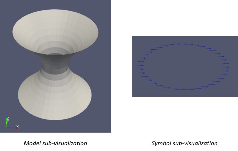
As already discussed in the OUTPUT-IMAGE function, a SesamX field is characterized by its nature: it can be a scalar, a vector or a tensor field. And this field nature drives the kind of symbol used in the visualization:

• a scalar field is always represented with points.
• a vector field is always represented with arrows. The direction of the arrow gives the direction of the vector, and the size of the arrow is proportional to the vector magnitude.
• a tensor field is always represented by 3 lines. The direction of each line gives the principal directions of the tensor, and the length of each line gives the absolute value of the principal values.

A mapping is a colored representation of some data on a sub-visualization. For instance, the translations at the nodes can be mapped on the model sub-visualization to get a colored representation of their magnitude.

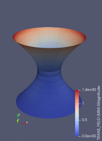
There are some rules that govern mappings:

• a mapping is either attached to nodes or to elements. We will see a bit further how to distinguish the attachment.
• a mapping can be a scalar mapping, a vector mapping or a tensor mapping. For instance, a translation mapping is a vector mapping.

Mappings can be applied through the options available in the properties panel, inside the “Display” section, and more precisely under “Coloring”.

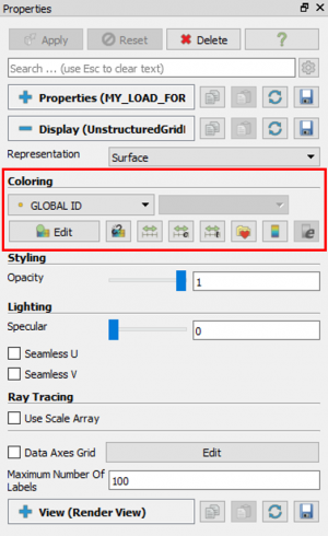
These options relate to the current sub-visualization selected in the pipeline browser. The “Coloring” lets you select which mapping you want to apply on the sub-visualization. The “Solid Color” mapping is always present. And depending on the sub-visualization, more mapping options are available.

For the model sub-visualization, you will always find 2 additional mappings:

• the nodes “Global ID” mapping, displaying the SesamX nodes ID on the model.
• and the elements “Global ID” mapping, displaying the SesamX elements ID on the model.

We will see later on how we can ask the SesamX viewer to add relevant mappings to the model sub-visualization.

For the symbols sub-visualization, you will always find one additional mapping: the mapping related to the field itself.

For a vector or tensor mapping, you can select the components or the magnitude to map on the visualization (obviously there is no such choice available for a scalar mapping).

Finally, you can distinguish a node mapping from an element mapping with the help of the symbol near the mapping name, as shown on the picture below.

This is pretty much what is needed to know about mappings. If you are looking for more information, do not hesitate to consult the Paraview documentation.

Besides visualization creation, the SesamX viewer allows you to edit an existing visualization. To active the edit mode, you need to check the “Edit Image” box in the SesamX viewer. Afterwards, once you have selected a visualization in the pipeline browser, the SesamX viewer edit section will update with the available options related to the visualization.

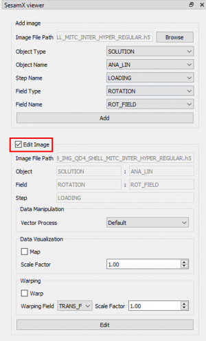
On this edit panel, you find first the information about the SesamX field related to the visualization. And next you find multiple options to control the visualization.

Depending on the field attachment (nodes or elements), the “Data Manipulation” section lets you specify the raw data used to plot the visualization.

For a field attached on the nodes or on the elements, you can select the process you want to apply to the field before plotting. A process is a function that takes a SesamX field on input and gives another field on output. For instance, you can apply a “Mises” process on stress data to get the Mises stress field.

The SesamX viewer proposes a set of predefined processes depending on the field nature. Currently for scalar and vector fields, only the “Default” process is available (i.e. the field is not processed). For tensor fields 3 processes are available:

• the “Default” process (as for scalar and vector fields).
• the “Mises” process computes the Von Mises criteria from the tensor components.
• the “Principal” process computes the tensor principal values.

Furthermore, for a field attached on the elements, you can select the locations inside the element where you want to visualize the data. You have 3 selectors to specify the desired location inside the element:

• the “Element Position” allows to select the desired location along the element dimension (“Center” or “Gauss”).
• the “Element Vertical Side”. This selector is used only for 1D and 2D elements. It allows you to select the location along the element thickness (“Bottom”, “Middle” or “Top”).
• the “Element Horizontal Side”. This selector is used only for 1D elements. It allows you to select the location along the element width (“Left”, “Middle” or “Right”).

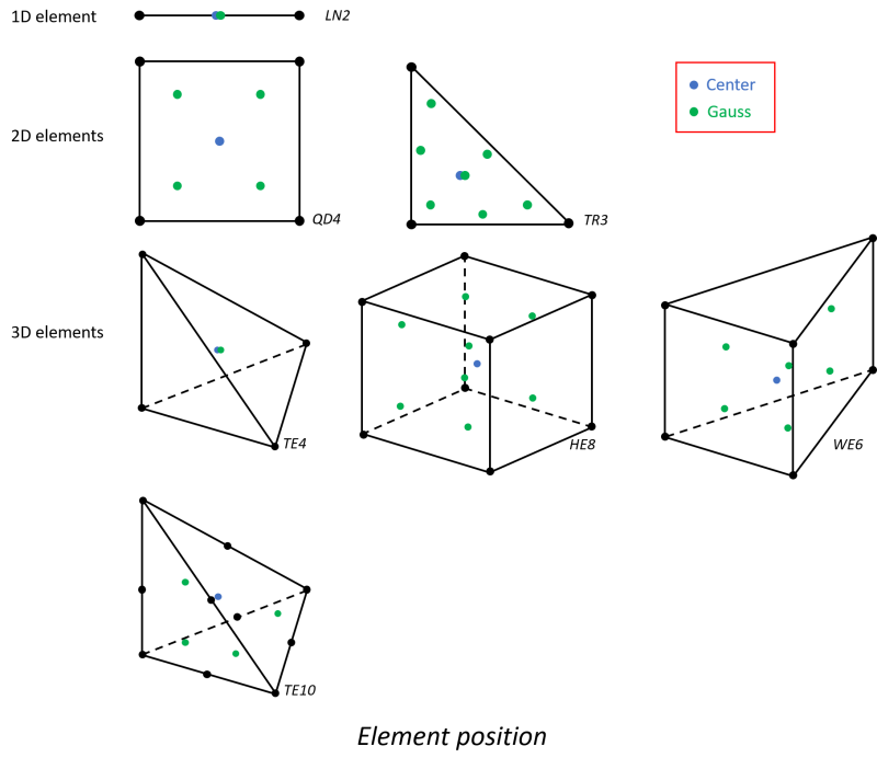
For instance, you can select to output stress data on a shell element at the center of the top face.

Using the data visualization section you can instruct the SesamX viewer to add a mapping of the field values on the model sub-visualization. For instance, as showcased in the following image, you can map the Mises stress on the model sub-visualization.

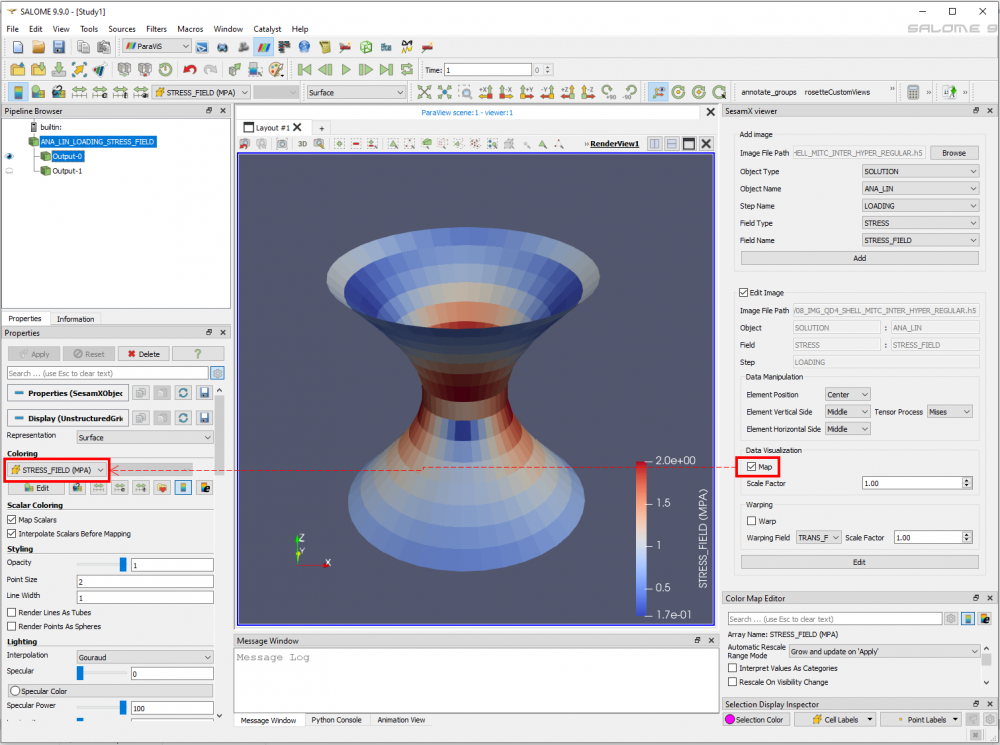
Furthermore, you can also provide the scale factor used to scale the symbols.

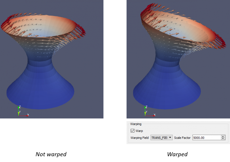
Finally the last section available is the “Warping” section. This section is available only when editing a visualization related to a solution field. It allows you to select a translation field on the solution, in order to warp the model and symbols sub-visualizations.

This part aims at providing some tips about Paraview that make things easier.

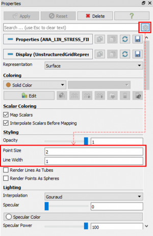
The line and point symbols (used for tensor and scalar fields) may sometimes be difficult to visualize. When necessary, you can increase the point size and the line width. To proceed, you need click on the gear icon in the properties panel, which shows hidden options. Then under the styling section you can control the “Point Size” and “Line Width” parameters.

• SesamX installation procedure
• SesamX OUTPUT-IMAGE function
• Pre-processing a SesamX model

• Paraview project website: Paraview website